PSO and GA Optimization Methods Comparison on Simulation Model of a Real Hexapod Robot
István Kecskés*, László Székács**, János C. Fodor*, Péter Odry***
*Obuda University, Budapest, Hungary
**University of Novi Sad, Novi Sad, Serbia
***College Dunaújváros, Dunaújváros, Hungary
kecskes.istvan@gmail.com, thewaslau@gmail.com, fodor@uni-obuda.hu, odry.peter@mail.duf.hu Abstract—The Szabad(ka)-II hexapod robot with 18 DOF is
a suitable mechatronic device for the development of hexapod walking algorithm and engine control [1, 2]. The required full dynamic model has already been built [3], which is used as a black-box for the walking optimizations in this research. The ellipse-based walking trajectory has been generated that was required by the low-cost straight line walking [4], and the purpose was to optimize its parameters. The Particle Swarm Optimization (PSO) method was chosen for simple and effective working, which does not require the model’s mathematical description or differentiation. Previously the authors performed an evolutionary Genetic Algorithm (GA) optimization for a similar trial case [5], and posed the principles of the quality measurement of hexapod walking [4, 5]. The same visual evaluation and comparison was applied in this paper for the results of both optimization methods. PSO has produced better and faster results compared to GA.
I. INTRODUCTION
The current research is a part of the Szabad(ka)-II hexapod walking robot’s development [1-6]. In the phase of building a hexapod robot the aim was to simulate the robot motion and optimize the drive parameters. In order to obtain optimal parameter values which can be used for the building or design of a real robot, a proper robot model is required. Our simulation model was introduced in [3], which is a detailed kinematic and dynamic model of the real Szabad(ka)-II robot. The aim of this model is to simulate the walking and measure its quality (named also performance) in comprehensive situations. Working with experiments instead of simulations is not a good choice for critical or complex industrial applications [9]. One of the fields where the robot model is used as a black-box is the categorization and optimization of the parameters which influence hexapodal gaits [5].
A. Performance Measurement – Fitness Function System parameters can be chosen correctly if one or more goals are defined. Generally these goals are [5]: a) achieving maximum speed of walking with as little electric energy as possible, b) keeping the minimal torques on the joints and gears, c) maintaining the currents of the engines discursive and spiky as little as possible, d) letting their variation be as small as possible while walking, and e) keeping the robot’s body acceleration at a minimum in all three dimensional directions.
The chosen robot's walking optimality is measured by a certain fitness function. The optimal parameter set consists of values in which the fitness function reaches its minimum or maximum value. In the previous research a
fitness function was already defined and used for the same problem [5]. This was modified in this case in order to obtain the results in accordance with our demands (1):
a) The averaged velocity was quadraticly taken into account in order to emphasize it at least as such as the small energy consumption and the small accelerations, i.
e. these two aspects influence the system oppositely.
b) The inverse of the fitness function described in [5]
was defined. In this research the optimum refers to the maximum value, where the zero-maximum domain was defined instead of the minimum-infinity domain.
0.03
100000 2
ACC LOSS ANG
ACC GEAR WALK
X
Z F
F F E
F V (1)
Where VX - the average walking speed (in direction X); EWALK - electric energy is needed for crossing unit distance;FGEAR - root mean square of the aggregated gear torques; FACC - root mean square of acceleration of the robot’s body; FANGACC - root mean square of angular acceleration of the robot’s body; ZLOSS - loss of height in direction Z during the walk. More detailed description of this fitness function can be found in [5, 6].
B. Experimental case
The straight-line hexapod walking on even ground is the simplest and most linear case. It has been assumed that in such case probably the robot goes for a farther target point, without any maneuver and other operations. Thus the most important task will be to achive a fast and low- cost (low energy consumption) locomotion. The presented fitness function (1) expressed the quality measurement of these features.
For the mentioned walking a three-dimensional ellipse- based trajectory curve was generated which defines the feet’s (end of the extremity) desired cyclic movement in relation to the robot body. More detailed description of this elliptic trajectory calculation can be found in [4].
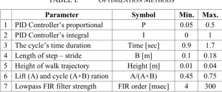
Both the trajectory curve and the driving motor controller’s behavior directly influence the real or simulated movement. Therefore the PI motor controller and the parameters of the mentioned trajectory have been chosen, this can be seen in Table I. The lower (min.) and upper (max.) bounds of these parameters were defined empirically in the most cases. Except the upper bound of the fourth “length of the step” (B) parameter is given by the structural dimension of the robot.
TABLE I. OPTIMIZATION METHODS
Parameter Symbol Min. Max.
1 PID Controller’s proportional P 0.05 0.5
2 PID Controller’s integral I 0 1
3 The cycle’s time duration Time [sec] 0.9 1.7 4 Length of step – stride B [m] 0.1 0.18 5 Height of walk trajectory Height [m] 0.01 0.04 6 Lift (A) and cycle (A+B) ration A/(A+B) 0.45 0.75 7 Lowpass FIR filter strength FIR order [msec] 4 300 Since the change of these parameters will influence the optimal values of the other parameters – that is, parameters are not independent – that’s why the optimal parameter set should be found in the multi-dimensional space. Naturally, parameters can be grouped, meaning that not all parameters have to be monitored simultaneously, only those that have significant influences on one another.
We ran the selected optimization algorithms on these correlative parameter groups.
II. OPTIMIZATION METHODS
Such optimization methods have been searched and compared that are adequate for the walking and driving optimization on the Simulink model of Szabad(ka)-II as a non-differentiable black-box. Because of the influence of the black-box object on the optimization we don't know whether the function that is to be optimized is convex, concave or differentiable. Therefore neither the techniques that give local solutions nor the gradient based methods is an option. Furthermore, it is an important aspect to receive the results quickly, due to the complexity of the model, one iteration takes 2-4 minutes on an Intel-i7-2600K processor. Table II details the methods that meet the criteria outlined above.
TABLE II. OPTIMIZATION METHODS
Method Convergence Characteristics Genetic
algorithm (GA) No convergence proof [10]
Stochastic Iterations Automatic initial populations or user supplied, or both[10]
Mixed-Integer Optimization [19]; Multiobjective [10]
Particle Swarm Optimization (PSO)
No convergence proof to the global optimum [25]
Stochastic Iterations Automatic initial populations or user supplied
Simulated Annealing (SA) [9]
Proven to converge to global opt. for bounded problems with very slow cooling schedule [10]
Stochastic Iterations
User supplied initial population [10]
Pattern Search (PA)
Proven convergence to local optimum [10]
Deterministic Iterations User supplied initial population [10]
Non-smooth optimization by Mesh-Adaptive Direct search (NOMAD)
Hypothetic convergence to Second-order Stationary Points [15]
Stochastic Iterations;
Automatic initial populations or user supplied; Categorical variables, discrete; Mixed variables optimization; Bi- objective; Mixed variables optimization[30];
In this research the PSO method was chosen, because of its speed, and its simple adjustability (details in II. B).
Comparison is made with GA, because that method [10]
has been thoroughly experienced, both methods tested
under the same conditions. It was also a criteria that the method has a Matlab implementation, which can be easily parallelized too.
A. Genetic Algorithm (GA)
The genetic algorithm uses a collection of possible solutions for a specific problem, using various strategies it groups them, then picks the more optimal results, creates new files and proceeds to an acceptable (maybe optimal) result [34].
The greatest advantage is that the algorithm is problem independent. In addition, unlike many other optimization methods, in many cases, it reaches the desired solution much faster [11]. It's considerable advantage is that it is parallel, multiple solutions are tested in the same time, can work with large-scale search spaces, 1000 bit or larger space is not uncommon, i.e. where the number of options is over 21000 [11]. Performs well in situations [13, 21-23]
where the fitness function is complex, not continuous, and full of errors [11]. Works without knowing the original problem, can produce solutions, so that does not use its properties. Thus the method is perfectly suitable for situations where this problem can’t be described but can value the results [11].
Disadvantage is that for specific optimization problems and problem instances, other optimization algorithms may find better solutions than genetic algorithms, but in most cases, a sufficiently good solution can be constructed with it [11]. Without the problem’s thorough knowledge, it is difficult to give an effective fitness function and fine-tune the parameters. Using guesses or solutions from a previous optimization, one must assume of what value should be changed in order to achieve a better approximation [11]. If it’s nearly impossible to find an adequate setup for the problem, than ultimately we can use a higher optimization to setup the parameters.
These advantages and disadvantages were observed in the previous [5] and current research too: a) Analytical evaluation of any sort wasn’t needed to be performed on the target model, only running the simulation; b) the time- consuming calculation could be easily sped up using parallelized computing; c) the resulted optimum depends on the optimization method’s parameters; d) in case of not comprehensive fitness function the result may be unexpectedly false.
GA’s most important parameters [17]:
Population Size – default value is 20, if the problem has many variables, it is advisable to use larger populations. For more complex problems using at least 100 is recommended [24].
Elite Count – default value is 2, it might be appropriate to increase with number of population.
Crossover Function – default value is scattered, alternatives: one-point, two-point, heuristic, etc.
There’s no standard process for choosing the appropriate method. [18][24]
Crossover Fraction – default value is 0.8, recommended to keep in (0.7, 0.9) interval. [24]
B. Particle Swarm Optimization (PSO)
Swarm intelligence describes the collective behavior of decentralized, self-organized systems, natural or artificial [31]. Particle swarm optimization (PSO), is one of the
most important swarm intelligence paradigms [32]. The PSO uses a simple mechanism that mimics swarm behavior in birds flocking and fish schooling to guide the particles to search for globally optimal solutions [33].
Each individual of the swarm describes a solution in the search space. Each particle knows the best previous value of their neighbors and of course himself (the current local optimum) and best value achieved by the swarm (the current global optimum). With every step, the particles modify their position in the previous local and global optimum as well as in combination with current or past situation. This algorithm uses random values in the process [12, 14, 20].
The algorithm's most important part is the update of the particles position and velocity [12].
) (t v Δt (t) x ) (t x
(t)]
[g(t)-x r (t)]+c [p(t)-x r (t)+c v w ) (t v
i i
i
i i
i i
1 1
1 1 1 2 2
(2)
Where w is called the inertia weight, c1 and c2 are weights on the attraction towards the particle’s own best known position p and the swarm’s best known position g.
These are also weighted by the random numbers r1 and r2
between (0,1).
Advantages are that it is intelligent, fast, simple and robust. Has no overlapping and mutation calculation, therefore a particle is not tested multiple times [25].
Performs well in situations [13], where the objective function is complicated and not continuous.
Disadvantages are that the method easily suffers from the partial optimism, which causes the loss of accuracy at the regulation of its speed and the direction. The method is unable to work out the problems indefinable in a coordinate system [25].
There is no built-in PSO algorithm in Matlab, therefore external sources exploration was needed [27-29].
Considering their characteristics for the first try was chosen to implement the own one [27]. Easy to learn, has the ordinary Matlab-like syntax, and has only the necessary options. The other two implementations [28, 29]
are better documented; due to their complexity it is understandable and also required. They have more tools for analyzing problems; however setting them up for different problems is more time-consuming.
Different problems need different setup. However the process performs surprisingly well with the default values if a problem is not overcomplicated. Important parameters, which are worth altering:
Inertia Weight (w) – tests [16] show that the value should be linearly decreasing between 1 and 0.3. So in the chosen implementation [27] the value 0.9 should be suitable. [7]
Cognitive Attraction, Social Attraction (c1, c2) – default values in order (0.5, 1.5). The practice shows, that the sum of these values should be between 2 and 4, and c2 should be bigger than c1. [7][26]
Populations – low number of population (0-15) is not suitable, the ideal value starts from 20 [16]. If the problem has many variables and/or needs bigger search space, it’s advisable to use bigger population.
Generations – number of generations should be set as high as possible. The algorithm will stop after 50
stationary populations. Of course, this value and also the sensitivity can be adjusted.
III. RESULTS
For both methods the number of generation was selected to NG=50, and the population size was NP=40.
The other GA-specific parameters were: elite count EL=2, the crossover function was one-point, the crossover fraction CF=0.88. The other PSO-specific parameters were: inertia weight w=0.9, cognitive attraction c1=0.5, social attraction c2=1.5. These parameters were selected partly from the literature [7, 8, 16, 17], partly from own experience.
In the initial state of the chosen simulation case, the robot’s bottom point was 1mm above the ground, the legs were set to the initial points of the desired trajectories. The simulation time was selected for only three seconds in order to hasten the runtime as much as possible, but at least to let simulate one and a half walking cycle. The ground was even with 0.9 friction constant.
The results of three optimization cases have been compared:
a) GA-2010-P, run GA method with results published in 2010 [5], but then the PID controller parameters were not included into the optimization, just there was a working P controller.
b) GA-2013-PI, run GA during current research based on parameters in Table I.
c) PSO-PI, run PSO during current research based on parameters in Table I.
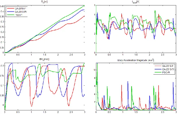
The Table III comprises of the fitness evaluation’s (1) detailed partial results for these three cases. The used PSO gave the best results with a prominent velocity and the smallest electric energy consumption. The torques and the robot-body’s accelerations have similar magnitude for all three cases, moreover which are acceptably small. Since the velocity was more emphasized quadraticly compared to earlier fitness function [5] the current results exactly show the expected form. Fig. 1 compares the mentioned simulation results and it can be apparently observed that the better fitness value accompanied with the more linear walk-direction movement prevails, i.e. its velocity has marginal fluctuation. Herewith a typical walking problem of the Szabad(ka)-II robot can be eliminated.
TABLE III. RESULTS OF FITNESS FUNCTION
GA-2010-
P GA-2013-
PI PSO-PI Gear torques FGEAR
Nm 9.89 9.56 9.12Body acceleration FACC
m/s2
1.67 1.76 1.80 Body angular acceleration
rad/s2
FANGACC 17.0 16.5 17.2
Energy per meter EWALKWs/m 68.1 49.2 42.5 Loss of height ZLOSS
m -0.00684 -0.00708 -0.00733 Mean velocity VXm/s 0.118 0.139 0.152
Fitness value F 1.97 3.78 5.17
Number of function calls 1902 1902 645
Figure 1. Simulation results of walking characteristics based on three kinds of optimized parameters: top-left the body movement in X direction (BX), bottom-left its velocity (BVX), top-right the aggregated motor current (ISUM), bottom-right the magnitude of body 3D acceleration
Figure 2. Simulated trajectory curves resulted by three optimization cases and the real Szabad(ka)-II robot A. Visual Evaluation of the Optimization Results
During the walking parameters’ optimizing process, the main issue was to determine the fitness function, i.e. what counts as proper or optimal walking. However, the emphasis primarily was put on the evaluation of the results and the measurement of their reliability.
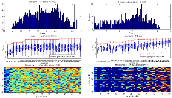
Since both the GA and PSO run the object function in two-dimensional form, i.e. the number of generation and the population size, thus the same presentations can be created. The Fig. 3 shows the evolution of the fitness values during the generations, which partly presents when
and how much the fitness improved, partly shows the evolvement from the best item in initial random population to the final aggregated best fitness. Practically only this increment counts the beneficial performance of the optimization, not the value of the optimum point itself.
B. Parameter Convergence Rate
Generally a multi-parameter optimization is required, where M is the number of parameters, and such a parameter combination (namely a gene with M dimensions) is to be found where the specified fitness function gives the best value. The result of the GA or PSO
is a pair consisting of a parameter combination arranged in a matrix (item p, matrix P) and the corresponding fitness value (item f, matrix F), see equation (3). These matrix dimensions are the number of generations (NG) and the population size (NP). Fig. 3 shows the fitness values in such a matrix form in the bottom graph; while the top graph includes the histogram of fitness values; and the middle graph illustrates the changing of fitness distribution during generations and the increasing of fitness maximums during generations.
p,f
M
PNGNPM,FNGNP (3)In order to measure and present the convergence of certain parameters the fitness thresholds (TF) have been determined and divided into N number of logarithmic scale between the minimum and maximum of the fitness values (4).
1 1 20 ln 1 exp min max
min ..
1
N F i
F F
N i TF
(4) For every item of the mentioned fitness threshold those parameter values can be selected from all the P matrix, where the fitness value pairs are greater or equal to this threshold value (for each parameter separately
M
m1,2,.., ). The standard deviation (PmSTD) can be calculated on this selected parameter set (5).
i f
p
m f T
i
PSTDm SD | F (5)
2
1 1
m
STD m STD
P m P
CR (6)
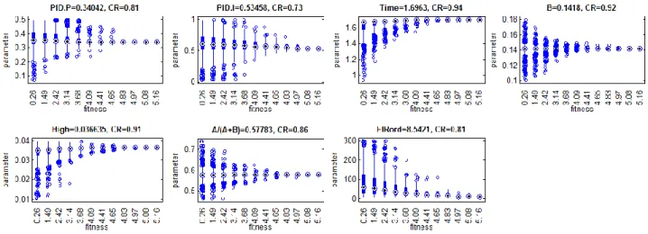
If this parameter deviation decreases to zero while the fitness threshold increases, it can be assumed that this parameter converges toward the current optimum. To express this convergence rate (CR) a specific simple expression has been defined (6). Fig. 4 illustrate parameter convergence with the calculated convergence rate for the GA and PSO results, where N=12. The parameters do not converge always toward an optimum with equal intensity, while the fitness value increases. Vertically, Fig. 4 shows the distribution of parameter values, and horizontally the increasing fitness threshold. A certain convergence rate (CR) and a confidence interval for a particular fitness threshold can also be determined for each parameter. In case if the convergence rate is small or this interval is relatively wide, the obtained optimum cannot be considered as reliable, or this parameter does not affect the fitness function i.e. to the subject of this optimization.
Figure 3. Visualized results of GA (left column) and PSO (right column) IV. CONCLUSION
The three examined and compared results (optimums) are not the same, they specify different parameters with different fitness values. If these optimization processes were called more times, they would probably not reach the same result, in other words, they would converge only toward a local optimum point. The obtaining of the global optimum required a comprehensive search with other suitable or mixed methods, maybe it needs applying more instances of running, with different parameterized runs.
In spite of this, the best given result - by PSO method - is currently acceptable and makes a significant headway compared to the previous research. It can be concluded from the current comparison that the used PSO algorithm is more suitable for this complex problem than the used GA implementation.
In the future a more comprehensive optimization of the robot driving is planned, with the aim to find the best effective multi-parameter optimization method, instead of the exact single timely determination of the optimum.
Figure 4. Parameter convergence from PSO
ACKNOWLEDGMENT
Grateful acknowledgments to Obuda University for financing the conference registration fee of this publication.
REFERENCES [1] www.szabadka-robot.com
[2] Ervin Burkus, Peter Odry: Autonomous Hexapod Walker Robot
“Szabad(ka)”, Acta Polytechnica Hungarica, Vol 5, No 1, 2008, pp 69-85, ISSN 1785-8860
[3] István Kecskés, Péter Odry: Full Kinematic and Dynamic Modeling of “Szabad(ka)-Duna” Hexapod, SISY 2009, pp:215- 219, ISBN: 978-1-4244-5348-1
[4] I. Kecskés, P. Odry: Walk Optimization for Hexapod Walking Robot, CINTI 2009, pp265-277
http://conf.uni-obuda.hu/cinti2009/25_cinti2009_submission.pdf [5] Z. Pap, I. Kecskés, E. Burkus, F. Bazsó, P. Odry: Optimization of
the Hexapod Robot Walking by Genetic Algorithm, SISY 2010, pp 121-126, ISBN: 978-1-4244-7394-6
[6] István Kecskés, Péter Odry: Protective Fuzzy Control of Hexapod Walking Robot Driver in Case of Walking and Dropping, Springer, 2010, Volume 313/2010, pp 205-217, DOI:10.1007/978- 3-642-15220-7_17
[7] E. Bonabeau, M. Dorigo, G. Theraulaz: Swarm intelligence from natural to artificial systems, Oxford University Press, 1999, ISBN 0-19-513158-4
[8] Magnus Erik Hvass Pedersen: Good Parameters for Particle Swarm Optimization, Hvass Laboratories, Technical Report no.
HL1001, 2010
[9] Radu-Emil Precup, Radu-Codrut David, Emil M. Petriu, Mircea- Bogdan Radac, Stefan Preitl, János C. Fodor: Evolutionary optimization-based tuning of low-cost fuzzy controllers for servo systems, 2013
[10] www.mathworks.com/products/global-optimization/index.html [11] Raffai Tamas: Genetikus Algoritmusok az optimalizalasban [12] Magnus Erik Hvass Pedersen: SwarmOps for MatlabNumeric &
Heuristic Optimization Source-Code Library for Matlab The Manual, 2010
[13] Pakize Erdogmus and Metin Toz: Heuristic Optimization Algorithms in Robotics, Serial and Parallel Robot Manipulators - Kinematics, Dynamics, Control and Optimization, Dr. Serdar Kucuk (Ed.), ISBN: 978-953-51-0437-7, InTech, DOI:
10.5772/30110, 2012
[14] Singiresu S. Rao: Engineering Optimization: Theory and Practice, Fourth Edition, ISBN-10: 0470183527, ISBN-13: 978- 0470183526, 2009
[15] Mark A. Abramson, Charles Audet: Convergence of Mesh Adatptive Direct Search to Second-order Stationary Points, SIAM
[16] J. Kennedy and R. Eberhart: Particle Swarm Optimization, Proc.
of IEEE International Conf. on Neural Networks IV, pp. 1942–
1948, 1995.
[17] Roger L. Wainwright: Introduction to Genetic Algorithms Theory and Applications, The Seventh Oklahoma Symposium on Artificial Intelligence, 1993
[18] David B. Fogel, Lauren C. Stayton: On the effectiveness of crossover in simulated evolutionary optimization, Biosystems Volume 32, Issue 3, pp 171–182, 1994
[19] http://www.mathworks.com/help/gads/ga.html#inputarg_IntCon [20] Balogh Sándor: Többszempontú gazdasági döntéseket segíto
genetikus algoritmus kidolgozása, 2009
[21] Fozia H. Khan, Nasiruddin Khan: Solving TSP problem by using genetic algorithm, IJBAS/IJENS, pp79-88, 2009
[22] Thijs Urlings, Rubén Ruiz: Genetic algorithms for complex hybrid flexible flow line problems, IJMHeur 1, pp 30-54, 2010
[23] P. Tormos, A. Lova: A Genetic Algorithm for Railway Scheduling Problems, Metaheuristics for Scheduling in Industrial and Manufacturing Applications, , pp 255-276, DOI: 10.1007/978-3- 540-78985-7_10, ISBN: 978-3-540-78984-0, 2008
[24] Siamak Sarmady: An Investigation on Genetic Algorithm Parameters, School of Computer Science, Universiti Sains Malaysia, 2007
[25] Qinghai Bai: Analysis of Particle Swarm Optimization Algorithm, Computer and Information Science 3(1): pp 180-184, 2010 [26] Hassan Azarkish, Said Farahat: Comparing the Performance of the
Particle Swarm Optimization and the Genetic Algorithm on the Geometry Design of Longitudinal Fin, World Academy of Science, Engineering and Technology, Vol.61, pp.836-839, 2012 [27] code.google.com/p/psomatlab/
[28] www.hvass-labs.org/projects/swarmops/matlab/
[29] www.georgeevers.org/pso_research_toolbox.htm [30] www.gerad.ca/nomad/Project/Home.html
[31] Lambert M. Surhone, Miriam T. Timpledon, Susan F. Marseken:
Swarm Intelligence, 2010, ISBN: 613035584X
[32] J. Kennedy, R. C. Eberhart, and Y. H. Shi, Swarm Intelligence.
San Mateo, CA: Morgan Kaufmann, 2001.
[33] Mehdi Neshat, Mehdi Sargolzaei, Azra Masoumi, Adel Najaran: A New Kind Of PSO: Predator Particle Swarm Optimization, 2012 [34] Jose Juan Tapia Valenzuela: A clustering genetic algorithm for
inferring protein-protein functional interaction sites, 2009