reaction–diffusion–convection equations

A new estimate of the minimal wave speed for travelling fronts in

reaction–diffusion–convection equations

Cristina Marcelli

and Francesca Papalini

Università Politecnica delle Marche, Via Brecce Bianche, Ancona, 60131, Italy Received 7 November 2017, appeared 13 February 2018

Communicated by Eduardo Liz

Abstract. In this paper we prove a new estimate of the threshold wave speed for trav- elling wavefronts of the reaction–diffusion–convection equations of the type

v_τ+h(v)vx= [D(v)vx]_x+f(v)

wherehis a convective term,Dis a positive (potentially degenerate) diffusive term and f stands for a monostable reaction term.

Keywords: reaction–diffusion equations, convective terms, travelling fronts, critical wave speed, singular boundary value problems, heteroclinic solutions.

2010 Mathematics Subject Classification: 35K57, 34B40, 34B16.

1 Introduction

Reaction–diffusion equations have been intensively investigated, since they model various biological and chemical phenomena. The simplest model in this context is the Fisher equation

∂v

∂τ = ^∂

2v

∂x² +v(1−v).

This equations has been subsequently generalized involving a general reaction term f(v)_, vanishing at v = 0 and v = 1, a general diffusive term D(v), which can be positive in [0, 1] (non-degenerate case), or positive in(0, 1] withD(0) = 0 (degenerate case), and a term H(v) to include possible convective phenomena

∂v

∂τ +^∂H(v)

∂x = ^∂

∂x

D(v)^∂v

∂x

+ f(v). (1.1)

A relevant class of solutions of equation (1.1) is that of travelling wave solutions (t.w.s.), that is solutions of the typev(τ,x):=u(x−cτ)for some one-variable functionuand real constant c, the wave speed.

BCorresponding author. Email: c.marcelli@univpm.it

In the monostable case, that is when the reaction term f is positive in(0, 1), it is known (see [11]) that there exists a threshold wave speed c^∗ such that equation (1.1) supports travelling wave solutions having speedcif and only if c≥c^∗. The importance of the valuec^∗ is due to the fact that in many cases the t.w.s. having speedc^∗ is the limit profile, for large times, of the solutions of the equation (1.1) (see, e.g., [3,6,7,9]).

For the valuec^∗ it is known the following estimate (see [11]) 2

q

(D(u)f(u))⁰(0) +h(0)≤c^∗ ≤2 s

sup

u∈(0,1]

D(u)f(u)

u + max

u∈[0,1]h(u) (1.2) whereh is the derivative of the one-variable function H. Estimate (1.2) is valid provided that the product function D· f is differentiable at u = 0. Notice that, when the convection is constant and the product function D· f is concave, then the previous estimate reduces to an equality: c^∗ =2p

(D(u)f(u))⁰(0) +h(0).

In [1] the following upper estimate was achieved for the threshold value c^∗, valid just in the case of no convective effects

1

4(c^∗)²≤ sup

u∈(0,1]

2 u²

Z _u

0 D(s)f(s)ds (1.3)

which improves the previous upper estimate (1.2) in the particular caseh ≡ 0. Such a result was achieved by means of a variational approach which seems to be not appropriate for equations involving convective effects.

A different variational principle was proposed in [2], where, under the further assumption thath∈C¹([0, 1]), it was proved that

c^∗≤ inf

α>0 sup

u∈(0,1]

α+ ¹

α

f(u)D(u)

u +h(u)

(1.4) which improves the upper estimate in (1.2), since the latter can be obtained by (1.4) taking

α= s

sup

u∈(0,1]

f(u)D(u)

u .

The value of c^∗ has been exactly determined for some special type of reaction–diffusion–

convection equations. For instance, in the case whenD(u) =u, f(u) =u(1−u)andh(u)≡0, thenc^∗ = ^√1

2 (see [15,16]). Other computations in presence of convective processes have been stated by Gibbs and Murray (see [14]) in the case D(u) =_1, f(u) = u(₁−u)_andh(u) = ku, for which it was showed (see also [11]) that

c^∗ =







2 fork≤2

2 k + ^k

2 fork>2.

Moreover, in [5] it was considered the equation

u_t+βu^ku_x = (αu^ku_x)_x+γu(₁−u^k)_,

withα ≥ 0, β, γ≥ 0 and k > 0 given constants, for which the authors proved that the value ofc^∗ is the following

c^∗ = ^β+^pβ²+4αγ(k+1) 2(k+₁) ^.

Finally, in the case when f(u) = u^m(1−u), D(u) = h(u) ≡ 0, the function c^∗ = c^∗(m) has been studied in [4], by means of asymptotical expansions as m→+_∞.

However, the exact computation of c^∗, or the study of its properties related to some pa- rameters of the equations, can be carried on just for special equations, for which the explicit solution is known. For general equations the value ofc^∗ has to be estimated.

The aim of this paper is to prove the following new upper estimate, valid also for equations involving convective effects,

c^∗ ≤2 s

sup

u∈(0,1]

1 u

Z _u

0

D(s)f(s)

s ds+ sup

u∈(0,1]

1 u

Z _u

0 h(s)ds (1.5)

and we show it improves both (1.2) and (1.3). Moreover, we also show that when his increas- ing, then the upper bound in (1.5) can be improved by the following

c^∗ ≤ sup

u∈(0,1]





 2

s 1 u

Z _u

0

D(s)f(s)

s ds+ ¹ u

Z _u

0

h(s)ds







(1.6)

We also present some extensions to other reaction–diffusion models, such as equations with bi-stable reaction terms (that is f is negative in (0,α)and positive in(α, 1)) or reaction–

diffusion–aggregation equations, in which the diffusivity Dcan also assume negative values.

For these type of equations, the estimate for the speedc^∗, obtained in the monostable reaction–

diffusion case, plays a relevant role.

2 Preliminaries

Let us consider equation (1.1). In what follows we will assume that f,D are continuous functions, defined in[_{0, 1}], both positive in the open interval(_{0, 1})_{, with} f(₀) = f(₁) =_{0, and} H ∈ C¹([0, 1]). In the whole paperh will denote the derivative ˙H. The diffusive term D can vanish atu=0 or/andu=1 (degenerate and doubly-degenerate case).

Assume that

f·Dis differentiable atu=_{0. (2.1)}

A functionv(τ,x)is said to be a travelling wave solution (t.w.s.) of (1.1) if there exists a real constantcand an one-variable function usuch thatv(τ,x) =u(x−cτ)for every(τ,x)in the domain of existence ofv. We are interested in t.w.s. connecting the two stationary statesv=0 and v = 1, that is satisfying u(−_∞) = 1 and u(+_∞) = 0. As it is immediate to verify, the profileuof a t.w.s. is a solution of the following second order boundary value problem

((D(u)u⁰)⁰+ (c−h(u))u⁰+ f(u) =0

u(−_∞) =1, u(+_∞) =0. (2.2)

Moreover, if a t.w.s. with speed c exists, then it is unique (up to shifts) and it is strictly decreasing whenever 0<u<1 (see [11]).

A travelling wave can be a solution in the classical sense (that is aC¹-function such that the productD(u)u⁰ isC¹as well, or in the weak sense (sharp solutions), that is solutions reaching one or both the equilibria at finite times and with slope possibly non zero. Sharp t.w.s. can appear when the diffusivity vanishes at u = 0 (degenerate case) and/or at u = _{1 (doubly}

degenerate case). We refer to [10] for a discussion about the characterization of the appearing travelling fronts.

The study of the existence or non-existence of t.w.s. is carried on by investigating the solvability of the following associate singular boundary value problem











˙

z= h(u)−c− ^f(u)D(u) z(u) z(0⁺) =z(1⁻) =0

z(u)<0 for everyu∈(0, 1).

(2.3)

where the dot stands for derivation with respect to the variable u. Indeed, since the profiles are strictly decreasing whenever 0<_u <1, then equation in (2.2) can be handled as a typical autonomous equation, settingz(u) =D(u)u⁰(t(u)), wheret(u)is the inverse function ofu(t). However, a careful analysis is needed regarding the behaviour at the equilibria, in order to obtain classical or sharp travelling fronts.

The aim of this paper is to improve the estimate of the threshold speed c^∗, so from now on we investigate the solvability of the boundary value problem (2.3), referring to [10] for the classification of the related travelling fronts. A key result providing a sufficient condition for the solvability of (2.3) is the following.

Theorem 2.1([13, Lemma 2.1]). If there exists a functionζ ∈ C¹(0, 1)such that ζ˙(u)≥ h(u)−c− ^f(u)D(u)

ζ(u) for every u∈(_{0, 1})

withζ(0⁺) = 0andζ(u) < 0 for every u ∈ (0, 1), then problem(2.3) admits a (unique) solution z satisfying

ζ(u)≤z(u)<0 for every u∈ (0, 1).

So, in order to prove the solvability of (2.3), it suffices to show the existence of a negative upper-solution for the equation in (2.3), approaching the origin.

3 The new estimates

We now state our main results.

Theorem 3.1. Assume(2.1). Let c>2

s sup

u∈(0,1]

1 u

Z _u

0

D(s)f(s)

s ds+ sup

u∈(0,1]

1 u

Z _u

0 h(s)ds. (3.1) Then problem(2.3)admits a solution.

Proof. Put

γ(u)_:=







f(u)D(u)

u for 0< u≤1, (f ·D)⁰(0) foru=0.

Since f(u)D(u)is differentiable atu=0, we get thatγis continuous in[_{0, 1}]_.

Put T:={(x,u)∈_R²: 0≤ x≤u≤1}and letG: T→_Rbe the function defined by

G(x,u):=





 1 u−x

Z _u

x γ(s)ds for 0≤ x<u≤1, γ(u) for 0≤ x=u≤1.

The function G is continuous in the compact triangle T. Indeed, the continuity is obvious at every point (x₀,u₀) ∈ T with x₀ < u₀, whereas as for the continuity at the points of bisectoru= xobserve that for every pair(x,u)∈T there exists a valueσ_x,u∈ [x,u]such that G(x,u) = γ(σ_x,u). So, if(x,u)→(u₀,u₀)for some u₀ ∈ [0, 1], we get σ_x,u → u₀ and then also G(x,u) =γ(σx,u)→γ(u₀) =G(u₀,u₀).

LetH :T→_Rbe the function defined by

H(x,u):=





 1 u−x

Z _u

x h(s)ds for 0≤ x<u≤1, h(u) for 0≤ x=u≤1.

Similarly to what we have done above, it is easy to show thatHis continuous on the triangleT.

Put M :=max_u∈[0,1]G(0,u)andN:=max_u∈[0,1]H(0,u). We have M = max

u∈[0,1]G(0,u) = sup

u∈(0,1]

G(0,u) = sup

u∈(0,1]

1 u

Z _u

0 γ(s)ds; (3.2) N= max

u∈[0,1]H(0,u) = sup

u∈(0,1]

H(0,u) = sup

u∈(0,1]

1 u

Z _u

0 h(s)ds. (3.3) By (3.1) we have ¹₄(c−N)² > M andc> N, so for someε>0 we have ¹₄(c−(N+ε))² >

M+εand c> N+ε. By the uniform continuity of the functions G and Hin the triangle T, there exists a realδ =δ_e>0 such that

G(x,u)≤ G(0,u) +ε≤ M+e for every x∈[0,δ]andu∈[x, 1]; (3.4) H(x,u)≤H(0,u) +ε≤N+e for every x∈ [0,δ]andu∈[x, 1]. (3.5) Let us choose a costant Lsuch thatM+ε < L< ¹₄(c−(N+ε))² and put

K:= ¹ 2

c−N−e+ q

(c−N−e)²−4L

.

Notice thatK²−(c−N−e)K=−LandK>0 sincec> N+ε. Moreover, by (3.4) we deduce that

G 1

n,u

= ¹

u−_n¹

Z _u

1 n

γ(s)ds <L for everyn> ¹

δ andu∈ _n¹, 1 . Therefore, for everyn> ¹

δ and everyu ∈ _n¹_{, 1we have} K²−(c−(N+ε))K= −L<− ¹

u− ¹_n

Z _u

n1

γ(s)ds implying

K

u− ¹ n

−c

u− ¹ n

+ (N+ε)

u− ¹ n

+

Z _u

1 n

γ(s)

K ds<0. (3.6)

Moreover, by (3.5) we get H

1 n,u

= ¹

u− ¹_n

Z _u

1 n

h(s)ds< N+ε.

So, by (3.6) we deduce K

u− ¹

n

−c

u− ¹ n

+

Z _u

1 n

h(s)ds+

Z _u

1 n

γ(s)

K ds<0, hence

−Ku>−K1 n +

Z _u

1 n

−c+h(s)− ^γ(s)

−K

ds=−K1 n+

Z _u

1 n

−c+h(s)− ^f(s)D(s)

−Ks

ds that is, putφ(u):=−Ku, for everyn> ¹

δ and every u∈ ¹_n, 1

, we have φ(u)>φ

1 n

+

Z _u

1n

−c+h(s)− ^f(s)D(s) φ(s)

ds. (3.7)

Therefore, putζ_n(u):=φ(_n¹) +Ru

1 n

−c+h(s)− ^f(s)D(s)

φ(s)

ds, we have ζ˙_n(u) =−c+h(u)− ^f(u)D(u)

φ(u) >−c+h(u)− ^f(u)D(u) ζn(u) andζ_n(¹_n) =φ(_n¹). Hence,ζ_n is an upper-solution for the problem







˙

z =−c+h(u)− ^f(u)D(u)

z foru∈ [¹_n, 1] z(¹_n) =φ(¹_n)

(3.8)

implying thatζ_n(u)>z_n(u)for everyu∈ _n¹, 1

, wherez_nis the (unique) solution of problem (3.8), in the interval₁

n, 1

. So, we conclude that

φ(u)>ζ_n(u)> z_n(u) for everyu∈ ¹_n, 1 .

Let us now continue each functionz_n in the whole interval [_{0, 1}] _{by setting}z_n(u) _:= φ(u) =

−Kufor every u∈[0,¹_n), denoting them again zn.

Let us now prove thatzn+1(_u)≤ zn(_u)_{for everyu}∈ [_{0, 1}]. By the construction ofzn, this is obvious for 0≤u ≤ _n¹, while, foru> ¹_n, sincez_n+1 1

n

<zn 1 n

, ifz_n+1(u¯) =zn(u¯)for some

¯

u∈ ¹_n, 1

, this contradicts the uniqueness of the solution of the Cauchy problem







˙

z=−c+h(u)− ^f(u)D(u)

z foru∈(¹_{n, 1}]_, z(u¯) =zn(u¯).

So,z_n+1(u)6= z_n(u)_{for every}u ∈ _n+¹_{1, 1, implying}z_n+1(u)< z_n(u)_{for every} u∈ ¹_{n, 1.} Summarizing, we have

−cu+

Z _u

0 h(s)ds≤z_n+1(u)≤zn(u)≤ −Ku for everyu∈ [0, 1].

Let Z(u):=lim_n→+_∞z_n(u). Notice that the sequence (z_n)_n is equibounded and equicon- tinuous in each compact subinterval [u, 1˜ ], with ˜u > 0. Indeed, for n sufficiently large and everyu∈[u, 1˜ ]we have

−c+h(u)≤ z˙_n(u) =−c+h(u)− ^f(u)D(u)

z_n(u) ≤ −c+h(u) + ^f(u)D(u) Ku ,

hence the convergence of the sequence (zn)_n towards the function Z is uniform in every compact subinterval[u, 1˜ ], implying that

Z˙(u) =−c+h(u)− ^f(u)D(u)

Z(u) ^{for everyu}∈ (0, 1). Finally, being −cu+Ru

0 h(s)ds ≤ Z(u) ≤ −Ku, we have Z(0) = 0 and Z continuous at 0.

Therefore, by Theorem 2.1, problem (2.3) admits a solution.

When h is increasing, then the upper bound given by (1.5) can be improved by (1.6), as stated in the following result.

Theorem 3.2. Assume(2.1). If h is increasing and c> sup

u∈(0,1]





 2

s 1 u

Z _u

0

D(s)f(s)

s ds+ ¹ u

Z _u

0 h(s)ds







(3.9) then problem(2.3)admits a solution.

Proof. Let us fixu∈(0, 1]and consider the following trinomial in the variableλ:

λ²+

cu−

Z _u

0 h(s)ds

λ+u Z _u

0

f(s)D(s)

s ds. (3.10)

By (3.9) we can deduce that the discriminant of the trinomial (3.10) is positive, so, if λ₁(u), λ₂(u)are the two roots, put

φ(u):= ¹

2(λ₁(u) +λ₂(u)) = ¹ 2

_{Z u}

0 h(s)ds−cu

we get

φ²(u) +

cu−

Z _u

0 h(s)ds

φ(u) +u Z _u

0

f(s)D(s)

s ds <0 for every u∈(0, 1] and sinceφ(u)<0 for every u∈(0, 1]we infer

φ(u)>

Z _u

0

(h(s)−c) ds− ^u φ(u)

Z _u

0

f(s)D(s)

s ds for everyu∈(0, 1] (3.11) Let us now consider the functionψ(u):= _| ^u

φ(u)| = ²

c−_u¹R_u

0 h(s)ds,u∈(0, 1]. Sincehis increasing, also the functionu7→ _u¹Ru

0 h(s)dsis increasing, and so alsoψdoes. Therefore,

− ^u φ(u)

Z _u

0

f(s)D(s)

s ds=ψ(u)

Z _u

0

f(s)D(s)

s ds

≥

Z _u

0 ψ(s)^f(s)D(s)

s ds

= −

Z _u

0

f(s)D(s) φ(s) ^ds

and taking (3.11) into account we get φ(u)>

Z _u

0

h(s)−c− ^f(s)D(s) φ(s)

ds for every u∈(0, 1]. (3.12) Hence, putξ(u):=Ru

0 h(s)−c− ^f(s)D(s)

φ(s)

ds, we have ξ˙(u) =h(u)−c− ^f(u)D(u)

φ(u) > h(u)−c− ^f(u)D(u)

ξ(u) ^{for everyu}∈(0, 1]

with ξ(0⁺) = 0 and ξ(u) < φ(u) < 0 for every u ∈ (0, 1]. So, by virtue of Theorem 2.1, problem (2.3) admits a solution.

Remark 3.3. Notice that estimates (1.5) and (1.6) are not comparable, since when h is in- creasing the upper bound given by (1.6) can be strictly less than the one given by (1.5), as Example4.4 in the next section shows. Instead, the validity of (1.6) for a generic convective termh, not necessarily increasing, remains an open problem.

4 Comparisons with the previous known estimates

In order to compare the various available estimates forc^∗, it is convenient to discuss separately the case of equations without convection and those with convection.

4.1 Comparison for reaction–diffusion equation (no convective effects) Observe that in this case (1.5) and (1.6) provide the same upper bound:

c^∗ ≤2 s

sup

u∈(0,1]

1 u

Z _u

0

f(s)D(s)

s ds (4.1)

which obviously improves the one given by (1.2), by the mean value theorem. Moreover, in this case the upper bound in (1.4) becomes

inf

α>0

sup

u∈(0,1]

α+ ¹

α

f(u)D(u) u

= inf

α>0 α+ ¹ α sup

u∈(0,1]

f(u)D(u) u

!

=2 s

sup

u∈(0,1]

f(u)D(u) u that is (1.4) furnishes the same upper bound as (1.2).

Finally, the next result states that (4.1) improves also the upper bound given by (1.3) (which has not an analogous version for reaction–diffusion–convection equations).

Theorem 4.1. Let f , D be satisfying assumption(2.1). Then, sup

u∈(0,1]

1 u

Z _u

0

f(s)D(s)

s ds ≤ sup

u∈(0,1]

2 u²

Z _u

0 f(s)D(s)ds. (4.2) Moreover, if relation(4.2)holds as an equality then necessarily

sup

u∈(0,1]

1 u

Z _u

0

f(s)D(s)

s ds = sup

u∈(0,1]

2 u²

Z _u

0 f(s)D(s)ds= (D f)⁰(0). (4.3)

Proof. For eachu∈(0, 1]let us consider the functions G(u):= ¹

u Z _u

0

f(s)D(s)

s ds, H(u):= ¹ u²

Z _u

0 f(s)D(s)ds and

T(u):=u(G(u)−H(u))−

Z _u

0 H(s)ds

=

Z _u

0

f(s)D(s)

s ds− ¹ u

Z _u

0 f(s)D(s)ds−

Z _u

0 H(s)ds.

Of course, Tis differentiable in (0, 1], with T⁰(_u) = ^f(u)D(u)

u + ¹

u² Z _u

0 f(_s)_D(_s)_ds− ^f(u)D(u)

u −H(_u) =_{0, for allu}∈(_{0, 1}]_, so T is constant in (0, 1]. Moreover, by the differentiability of the product function f(u)D(u) atu=0, we haveT(0⁺) =0. Therefore, T(u) =0 for allu∈ (0, 1], implying that

G(u) =H(u) + ¹ u

Z _u

0 H(s)ds, for all u∈(0, 1]. Hence,

sup

u∈(0,1]

G(u)≤ _sup

u∈(0,1]

H(u) + _sup

u∈(0,1]

1 u

Z _u

0

H(s)ds≤_{2 sup}

u∈(0,1]

H(u)_{, (4.4)} which proves inequality (4.2).

Moreover, if relation (4.2) holds as equality then by (4.4) we get that sup

u∈(0,1]

H(u) = sup

u∈(0,1]

1 u

Z _u

0 H(s)ds. (4.5)

Hence, the following two situations can occur:

sup

u∈(0,1]

H(u) = sup

u∈(0,1]

1 u

Z _u

0 H(s)ds = H(0⁺) = ¹

2(f D)⁰(0); (4.6) or

H(u)≤ ¹ δ

Z _δ

0 H(s)ds= sup

v∈(0,1]

1 v

Z _v

0 H(s)ds for everyu∈ (0,δ]. (4.7) When (4.6) holds, we have sup_u∈(0,1]G(u) = (f D)⁰(0), hence (4.3) holds. Instead, when (4.7) holds, then His constant in[0,δ], so

sup

u∈(0,1]

1 u

Z _u

0 H(s)ds= ¹ δ

Z _δ

0 H(s)ds= ¹

2H(0⁺) = ¹

2(f D)⁰(0) and (4.3) holds.

Remark 4.2. Notice that when (4.3) holds, all the estimates (1.2), (1.3) and (1.5) reduce to the equality c^∗ = ¹₂^p(f ·D)⁰(0). This situation occurs, for instance, when the product function f ·D is concave in [0, 1], or is concave in [0, ¯u] and convex in [u, 1¯ ], for some ¯u ∈ (0, 1). Theorem4.1states that when the right-hand side of the estimates is greater than the left-hand one, that is when c^∗ is just unknown, then estimate (1.5) is properly sharper then the other ones.

Example 4.3. Just to furnish a numerical example, note that for the very simple caseD(u) =u and f(u) =u(1−u), estimate (1.2) providesc^∗ ≤1, estimate (1.3) providesc^∗ ≤ ²₃√

2 ∼0.94, finally estimate (4.1) providesc^∗ ≤ ¹₂√

3∼ 0.87. However, for this special case the exact value of c^∗ is known: c^∗= ¹₂√

2∼0.71 (see [16]).

4.2 Comparison for reaction–diffusion–convection equations

Obviously, estimate (1.5) improves (1.2), by the mean value theorem, and (1.6) improves (1.5) in the case whenh is increasing. In this case, (1.6) provides a better upper bound than (1.5), as the following example shows. Moreover, the relation between (1.6) and (1.4) is unclear, but in the following example, (1.6) provides a better upper bound also with respect to (1.4).

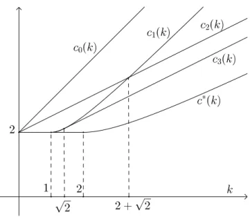
Figure 4.1: Graphics of the exact minimal speed c^∗(k) and the upper bounds c0(_k)(by (1.2)),c1(_k)(by (1.4)),c2(_k)(by (1.5)) and c3(_k)(by (1.6)).

Example 4.4. Let us consider the model studied by Gibbs and Murray: D(u) ≡ 1, f(u) = u(1−u) andh(u) = ku(k > 0), for which the exact value ofc^∗ is known (see Introduction).

Letc0(_k)_{, c1}(_k)_,c2(_k)_andc3(_k)respectively denote the upper bounds derived from estimates (1.2), (1.4), (1.5) and (1.6). As it is easy to check,c₀(k) =2+kandc₂(k) =2+¹₂k, and clearly c₂(k)<c₀(k). As forc₁(k), notice that for everyα>0 we have

sup

u∈(0,1]

α+ ¹

α

f(u)D(u)

u +h(u)

=α+ ¹ α

+ _sup

u∈(0,1]

k− ¹

α

u= (

α+k if α≥ ¹_k, α+ ¹

α if α≤ ¹_k. So,

c₁(k) = inf

α>0 sup

u∈(0,1]

α+ ¹

α

f(u)D(u)

u +h(u)

=

(2 ifk≤1, k+¹_k ifk≥1.

Hence, c₁(k) < c₀(k) for every k > 0, but c₁(k) > c₂(k) whenever k > 2+√

2. Finally, by simple computations one has

c₃(k) =















2 if 0≤ k≤1, k+ ¹

k if 1≤ k≤√ 2,

√ 2+ ¹

2k ifk≥√ 2,

and c₁(k) > c₃(k) for every k > 0. Hence, for every k > 0 we have c₃(k) < c₂(k) and c3(k)<c₁(k).

5 Extension to other reaction–diffusion models

The estimate for the threshold wave c^∗ for the reaction–diffusion–convection equations plays a relevant role also for other type of models. So, we now present the natural extension of known results which can be achieved taking estimate (1.5) into account. Of course, analogous results can be derived using (1.6) whenh is increasing.

5.1 Reaction–diffusion–convection with bi-stable reaction terms

Another well-known model for reaction–diffusion equations concerns the case of bi-stable reaction terms, that is when the continuous function f is assumed to be negative in(0,α)and positive in(α, 1)for someα∈(0, 1). In this case, it was shown that there exists a unique value

˜

csuch that equation (1.1) supports t.w.s. having speedc= c. As for the estimate of ˜˜ c, in [12]

it was proved the following estimate

−2 s

sup

u∈[0,α)

f(u)D(u) u−α

− max

u∈[0,α]h(u)≤c˜≤2 s

sup

u∈(α,1]

f(u)D(u) u−α

− min

u∈[α,1]h(u).

Such a relation has been obtained starting from estimate (1.2) for the mono-stable case. Using the same proof as in [12], taking the present estimate (1.5) into account, the estimate of ˜ccan be improved by the following

−2 s

sup

u∈[0,α)

1 α−u

Z _α

u

f(s)D(s) s−α ds

− sup

u∈[0,α]

1 α−u

Z _α

u h(s)ds ≤c˜

≤2 s

sup

u∈(α,1]

1 u−α

Z _u

α

f(s)D(s) s−α ds

− inf

u∈[α,1]

1 u−α

Z _u

α

h(s)ds. (5.1)

5.2 Extension to diffusion–aggregation models

In [8] it was proposed a model of diffusion–aggregation–reaction process (without convective effects), in which the diffusive term can assume negative values too, in order to describe the behaviour of a population tending to cluster into groups for some value of the density u.

Assuming the existence of a value β ∈ (0, 1)such that D(u)(β−u) > 0 for everyu ∈ (0, 1), u6= β, it was proved that there exists a threshold valuec^∗ such that equation

∂v

∂τ = ^∂

∂x

D(v)^∂v

∂x

+ f(v)

supports t.w.s. (classical or sharp) if and only if c≥c^∗, withc^∗satisfying the following upper estimate

1

4(c^∗)² ≤_max (

sup

0<u≤β

f(u)D(u)

u , sup

β≤u<₁

f(u)D(u) u−1

)

(5.2) obtained from the classical estimate (1.2) for the merely diffusive model. So, taking account of the present estimate (1.5), inequality (5.2) can be improved by

1

4(c^∗)²≤max (

sup

0<u≤β

1 u

Z _u

0

f(s)D(s)

s ds, sup

β≤u<1

1 1−u

Z ₁

u

f(s)D(s) s−1 ds

) .

References

[1] M. Arias, J. Campos, A. M. Robles-Pérez, L. Sanchez, Fast and heteroclinic solu- tions for a second order ODE related to Fisher–Kolmogorov’s equation,Calc. Var. Partial Differential Equations 21(2004), No. 3, 319–334. MR2094324; https://doi.org/10.1007/

s00526-004-0264-y

[2] R. D. Benguria, M. C. Depassier, V. Méndez, Minimal speed of fronts of reaction–

convection–diffusion equations,Phys. Rev. E (3)69(2004), No. 5, 031106, 7 pp.MR2096389;

https://doi.org/10.1103/PhysRevE.69.031106

[3] J. I. Díaz, S. Kamin, Convergence to travelling waves for quasilinear Fisher–KPP type equations,J. Math. Anal. Appl.390(2012), No. 1, 74–85.MR2885754;https://doi.org/10.

1016/j.jmaa.2012.01.018

[4] F. Dumortier, N. Popovi ´c, T. J. Kaper, The asymptotic critical wave speed in a family of scalar reaction–diffusion equations, J. Math. Anal. Appl. 326(2007), No. 2, 1007–1023.

MR2280959;https://doi.org/10.1016/j.jmaa.2006.03.050

[5] B. H. Gilding, R. Kersner, A Fisher/KPP-type equation with density-dependent diffu- sion and convection: travelling-wave solutions. J. Phys. A 38(2005), No. 15, 3367–3379.

MR2132716;https://doi.org/10.1088/0305-4470/38/15/009

[6] S. Kamin, P. Rosenau, Emergence of waves in a nonlinear convection–reaction–diffusion equation, Adv. Nonlinear Stud. 4(2004), No. 3, 251–272. MR2079814; https://doi.org/

10.1515/ans-2004-0302

[7] S. Kamin, P. Rosenau, Convergence to the travelling wave solution for a nonlinear reaction–diffusion equation, Atti Accad. Naz. Lincei Cl. Sci. Fis. Mat. Natur. Rend. Lincei (9) Mat. Appl.15(2004),No. 3–4, 271–280.MR2148885

[8] P. K. Maini, L. Malaguti, C. Marcelli, S. Matucci, Diffusion–aggregation processes with mono-stable reaction terms, Discrete Contin. Dyn. Syst. Ser. B 6(2006), No. 5, 1175–

1189.MR2224877;https://doi.org/10.3934/dcdsb.2006.6.1175

[9] L. Malaguti, S. Ruggerini, Asymptotic speed of propagation for Fisher-type degenerate reaction–diffusion–convection equations, Adv. Nonlinear Stud. 10(2010), No. 3, 611–629.

MR2676636;https://doi.org/10.1515/ans-2010-0306

[10] L. Malaguti, C. Marcelli, Finite speed of propagation in monostable degenerate reaction–diffusion–convection equations, Adv. Nonlinear Stud. 5(2005), No. 2, 223–252.

MR2126737;https://doi.org/10.1515/ans-2005-0204

[11] L. Malaguti, C. Marcelli, Travelling wavefronts in reaction–diffusion equations with convection effects and non-regular terms, Math. Nachr. 242(2002), No. 1, 148–164.

MR1916855; https://doi.org/10.1002/1522-2616(200207)242:1<148::AID-MANA148>

3.0.CO;2-J

[12] L. Malaguti, C. Marcelli, S. Matucci, Front propagation in bistable reaction–

diffusion–advection equations, Adv. Differential Equations 9(2004), No. 9–10, 1143–1166.

MR2098068

[13] L. Malaguti, C. Marcelli, S. Matucci, Continuous dependence in front propagation of convective reaction–diffusion equations,Commun. Pure Appl. Anal.9(2010), 1083–1098.

MR2610263;https://doi.org/10.1155/2011/986738

[14] J. D. Murray,Mathematical biology, Springer-Verlag, Berlin, 1993.

[15] F. Sánchez-Garduno, P. K. Maini, An approximation to a sharp type solution of a density-dependent reaction–diffusion equation, Appl. Math. Lett. 7(1994), No. 1, 47–51.

MR1349892;https://doi.org/10.1016/0893-9659(94)90051-5

[16] J. A. Sherratt, On the form of smooth-front travelling waves in a reaction–diffusion equation with degenerate nonlinear diffusion,Math. Model. Nat. Phenom. 5(2010), No. 5, 64–79.MR2681228;https://doi.org/10.1051/mmnp/20105505