Diﬀerential Equations and Dynamical Systems

(1)

Differential Equations and Dynamical Systems

P´ eter L. Simon E¨ otv¨ os Lor´ and University

Institute of Mathematics

Department of Applied Analysis and Computational Mathematics

2012

(2)

Chapter 1 Introduction

Preface

These lecture notes are based on the series of lectures that were given by the author at the Eötvös Loránd University for master students in Mathematics and Applied Math- ematics about the qualitative theory of differential equations and dynamical systems.

The prerequisite for this was an introductory differential equation course. Hence, these lecture notes are mainly at masters level, however, we hope that the material will be useful for mathematics students of other universities and for non-mathematics students applying the theory of dynamical systems, as well.

The prerequisite for using this lecture notes is a basic course on differential equations including the methods of solving simple first order equations, the theory of linear systems and the methods of determining two-dimensional phase portraits. While the basic existence and uniqueness theory is part of the introductory differential equation course at the Eötvös Loránd Universitynot, these ideas are not presented in these lecture notes.

However, the reader can follow the lecture notes without the detailed knowledge of existence and uniqueness theory. The most important definitions and theorems studied in the introductory differential equation course are briefly summarized in the Introduc- tion below. For the interested reader we suggest to consult a textbook on differential equations, for example Perko’s book [19].

Acknowledgement

The author is grateful to his colleagues at the Department of Applied Analysis and Computational Mathematics in the Institute of Mathematics at the Eötvös Loránd Uni- versity, who supported the creation of a dynamical system course at the University, and encouraged the efforts to make lecture notes electronically available to the students of the course.

(6)

The author appreciates the careful work of the referee, Tam´as Kurics, who provided detailed comments, identified errors and typos, and helped to increase distinctness and consistency of the notes.

The lecture notes were written in the framework of the projectTAMOP-4.1.2.A/1- 11/1, titled Interdisciplinary and complex development of digital curriculum for science master programmes.

(7)

1.1 Qualitative theory of differential equations and dynamical systems

The theory of differential equations is a field of mathematics that is more than 300 years old, motivated greatly by challenges arising from different applications, and leading to the birth of other fields of mathematics. We do not aim to show a panoramic view of this enormous field, we only intend to reveal its relation to the theory of dynamical systems.

According to the author’s opinion the mathematical results related to the investigation of differential equation can be grouped as follows.

• Deriving methods for solving differential equations analytically and numerically.

• Prove the existence and uniqueness of solutions of differential equations.

• Characterize the properties of solutions without deriving explicit formulas for them.

There is obviously a significant demand, coming from applications, for results in the first direction. It is worth to note that in the last 50 years the emphasis is on the numerical approximation of solutions. This demand created and motivated the birth of a new disci- pline, namely the numerical methods of differential equations. The question of existence and uniqueness of initial value problems for ordinary differential equations was answered completely in the first half of the twentieth century (motivating the development of fixed point theorems in normed spaces). Hence today’s research in the direction of existence and uniqueness is aimed at boundary value problems for non-linear ordinary differential equations (the exact number of positive solutions is an actively studied field) and initial-boundary value problems for partial differential equations, where the question is answered only under restrictive conditions on the type of the equation. The studies in the third direction go back to the end of the nineteenth century, when a considerable demand to investigate non-linear differential equations appeared, and it turned out that these kind of equations cannot be solved analytically in most of the cases. The start of the qualitative theory of differential equations was first motivated by Poincar´e, who aimed to prove some qualitative properties of solutions without deriving explicit formulas analytically. The change in the attitude of studying differential equations can be easily interpreted by the simple example ˙x= x, ˙y =−y. This system can be obviously solved analytically, the traditional approach is to determine the solutions as x(t) = e^tx0, y(t) = e^−ty₀. The new approach, called qualitative theory of differential equations, gives a different answer to this question. Instead of solving the differential equations it pro- vides the phase portrait as shown in Figure 1.1. This phase portrait does not show the time dependence of the solutions, but several important properties of the solutions can be obtained from it. Moreover, the phase portrait can be determined also for non-linear systems, for which the analytic solution is not available. Thus a system of ordinary differential equations is considered as a dynamical system, the orbits of which are to be

(8)

Figure 1.1: The phase portrait of the system ˙x=x, ˙y=−y, the so-called saddle point.

characterized, mainly from geometric or topological point of view. Based on this idea, the qualitative theory of differential equations and the theory of dynamical systems became closely related. This is shown also by the fact that in the title of modern monographs the expression ”differential equation” is often accompanied by the expression ”dynamical system”. A significant contribution to the development of qualitative theory was the invention of chaotic systems and the opportunity of producing phase portraits by numerical approximation using computers. The use of the main tools of qualitative theory has become a routine. Not only the students in physics, chemistry and biology, but also students in economics can use the basic tools of dynamical system theory. Because of the wide interest in applying dynamical systems theory several monographs were published in the last three decades. These were written not only for mathematicians but also for researchers and students in different branches of science. Among several books we men- tion the classical monograph by Guckenheimer and Holmes [11], an introduction to chaos theory [1], the book by Hale and Ko¸cak [12], by Hubbard and West [16], and by Perko [19]. Seydel’s book [22] introduces the reader to bifurcation theory. The emphasis in the following books is more on proving the most important and relevant theorems. Hence for mathematics student the monographs by Chow and Hale [8], by Chicone [7], by Hirsch, Smale and Devaney [15], by Robinson [20] and by Wiggins [27] can be recommended.

1.2 Topics of this lecture notes

In this section we introduce the mathematical framework, in which we will work, and list briefly the topics that will be dealt with in detail. The object of our study is the system of autonomous ordinary differential equations (ODEs)

˙

x(t) =f(x(t))

(9)

where x : R → Rⁿ is the unknown function and f : Rⁿ → Rⁿ is a given continuously differentiable function that will be referred to as right hand side (r.h.s). Most of the ordinary differential equations can be written in this form and it is impossible to list all physical, chemical, biological, economical and engineering applications where this kind of system of ODEs appear.

The solution of the differential equation satisfying the initial condition x(0) = p is denoted by ϕ(t, p). It can be proved that ϕ is a continuously differentiable function satisfying the assumptions in the definition of a (continuous time) dynamical system below.

Definition 1.1.. A continuously differentiable function ϕ : R×Rⁿ → Rⁿ is called a (continuous time) dynamical system if it satisfies the following properties.

• For all p∈Rⁿ the equation ϕ(0, p) =p holds,

• For all p∈Rⁿ and t, s∈R the relation ϕ(t, ϕ(s, p)) =ϕ(t+s, p) holds.

A dynamical system can be considered as a model of a deterministic process, Rⁿ is the state space, an element p∈Rⁿ is a state of the system, and ϕ(t, p) is the state, to which the system arrives after time t starting from the state p. As it was stated above, the solution of the above system of autonomous ordinary differential equations determines a dynamical system (after rescaling of time, if it is necessary). On the other hand, given a dynamical system one can define a system of autonomous ordinary differential equations, the solution of which is the given dynamical system. Hence autonomous ordinary differential equations and (continuous time) dynamical systems can be considered to be equivalent notions. We will use them concurrently in this lecture notes.

The above definition of the dynamical system can be extended in several directions.

One important alternative is when time is considered to be discrete, that is Z is used instead of R. This way we get the notion of (discrete time) dynamical systems.

Definition 1.2.. A continuous function ϕ : Z× Rⁿ → Rⁿ is called a discrete time dynamical system if it satisfies the following properties.

• For all p∈Rⁿ the equation ϕ(0, p) =p holds,

• For all p∈Rⁿ and k, m∈Z the relation ϕ(k, ϕ(m, p)) =ϕ(k+m, p) holds.

As the notion of (continuous time) dynamical systems was derived from autonomous ordinary differential equations, the notion of discrete time dynamical systems can be derived from difference equations. A difference equation can be defined by a map. Namely, let g :Rⁿ →Rⁿbe a continuous function and consider the difference equation (or recursion)

x_k+1 =g(x_k)

(10)

with initial condition x₀ = p. The function ϕ(k, p) = x_k satisfies the properties in the definition of the discrete time dynamical system. Thus a difference equation determines a discrete time dynamical system. On the other hand, if ϕ is a discrete time dynamical system, then introducing g(p) = ϕ(1, p) one can easily check that x_k = ϕ(k, p) is the solution of the recursionx_k+1 =g(x_k). This is expressed with the formulaϕ(k, p) = g^k(p), where g^k denotes the compositiong◦g◦. . .◦g k times. (Ifk is negative then the inverse function of g is applied.

Continuous and discrete time dynamical systems often can be dealt with concurrently.

Then the set of time points is denoted byTas a common notation forRandZ. In the case of continuous time the notion ”flow”, while in the case of discrete time the notion ”map” is used. The main goal in investigating dynamical systems is the geometric characterization of the orbits that are defined as follows. The orbit of a point p is the set

{ϕ(t, p) : t∈T}

that is a curve in the continuous case and a sequence of points in the discrete case.

After defining the main concepts used in the lecture notes let us turn to the overview of the topics that will be covered.

In the next section we show how the differences and similarities of phase portraits can be exactly characterized from the geometrical and topological point of view. In order to do so we introduce the notion of topological equivalence, that is an equivalence relation in the set of dynamical systems. After that, we investigate the classes determined by the topological equivalence and try to find a simple representant from each class. The main question is how to decide whether two systems are equivalent if they are given by differential equations and the dynamical system ϕ is not known. The full classification can be given only for linear systems.

Nonlinear systems are classified in Section 3. However, in this case only the local classification in the neighbourhood of equilibrium points can be carried out. The main tool of local investigation is linearization, the possibility of which is enabled by the Hartman–Grobman theorem. If the linear part of the right hand side does not determine the phase portrait, then those nonlinear terms that play crucial role in determining the equivalence class the system belongs to can be obtained by using the normal form theory.

The stable, unstable and center manifold theorems help in the course of investigating the local phase portrait around steady states. These theorems are dealt with in Section 4. The manifolds can be considered as the generalizations of stable, unstable and center subspaces introduced for linear systems. These manifolds are invariant (similarly to the invariant subspaces), that is trajectories cannot leave them. The stable manifold contains those trajectories that converge to the steady state as t → +∞, while the unstable manifold contains those points, from which trajectories converge to the steady state as t → −∞. The center manifold enables us to reduce the dimension of the complicated part of the phase space. If the phase portrait can be determined in this lower dimensional manifold, then it can also be characterized in the whole phase space.

(11)

Tools for investigating the global phase portrait are dealt with in Section5. First, an overview of methods for determining two dimensional phase portraits is presented. Then periodic solutions are studied in detail. Theorems about existence and non-existence of periodic solutions in two dimensional systems are proved first. Then the stability of periodic solutions is studied in arbitrary dimension. In the end of that section we return to two dimensional systems and two strong tools of global investigation are shown.

Namely, the index of a vector field and compactification by projecting the system to the Poincar´e sphere.

In the next sections we study dynamical systems depending on parameters, especially the dependence of the phase portraits on the value of the parameters. Methods are shown that can help to characterize those systems, in which a sudden qualitative change in the phase portrait appears at certain values of the parameters. These qualitative changes are called bifurcations. We deal with the two most important one co-dimensional bifurcations, the fold bifurcation and the Andronov–Hopf bifurcation, in detail.

An important chapter of dynamical systems theory is chaos. Our goal is to define what chaos means and investigate simple chaotic systems. The tools are developed mainly for discrete time dynamical systems, hence these are investigated separately in section 8. Methods for investigating fixed points, periodic orbits and their stability are shown.

We introduce one of the several chaos definitions and prove that some one dimensional maps have chaotic orbits. As a tool we introduce symbolic dynamics and show how can it be applied to prove the appearance of chaos.

The last section presents an extension of dynamical systems theory to systems with infinite dimensional phase space. This can typically happen in the case of partial differential equations. In that section semilinear parabolic partial differential equations are studied that are often called reaction-diffusion equations. The existence and stability of stationary solutions (that correspond to equilibrium points) is studied first. Then, an- other type of orbit, the travelling wave is studied that is important from the application point of view. For these solutions again the question of existence and stability is dealt with in detail.

(12)

Chapter 2 Topological classification of dynamical systems

The evolution of the theory of differential equations started by developing methods for solving differential equations. Using these methods the solution of different special differential equations can be given analytically, i.e. formulas can be derived. However, it turned out that the solution of systems of ordinary differential equations can be obtained analytically only in very special cases (e.g. for linear systems), and even in the case when formulas can be derived for the solutions, it is difficult to determine the properties of the solutions based on the formulas. For example, two dimensional linear systems can be characterized by plotting trajectories in the phase plane instead of deriving formulas for the solutions. It does not mean that the trajectories are plotted analytically, instead the main characteristics of the trajectories are shown, similarly to the case of plotting graphs of functions in calculus, when only the monotonicity, local maxima, minima and the convexity are taken into account, the exact value of the function does not play important role. Thus the construction of the phase portrait means that we plot the orbits of a system that is equivalent to the original system in a suitable sense, that somehow expresses that the phase portraits of the two systems ”look like similar”. In this section our aim is to define the equivalence of dynamical systems making the notion of ”look like similar” rigorous.

We will define an equivalence relation for dynamical systems ϕ : R× M → M. Then the goal is to determine the classes given by this equivalence relation, to find a representant from each class, the phase portrait of which can be easily determined, and finally, to derive a simple method that helps to decide if two systems are equivalent or not.

(13)

2.1 Equivalences of dynamical systems

Two dynamical systems will be called equivalent if their orbits can be mapped onto each other by a suitable mapping. First we define the classes of mappings that will be used.

The equivalence relations for discrete and continuous time dynamical systems will be defined concurrently, hence we use the notation T forR or for Z.

Definition 2.1.. Let M, N ⊂ Rⁿ be open sets. A function h : M → N is called a homeomorphism (sometimes a C⁰-diffeomorphism), if it is continuous, bijective and its inverse is also continuous. The function is called a C^k-diffeomorphism, if it is k times continuously differentiable, bijective and its inverse is also k times continuously differentiable.

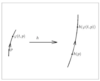
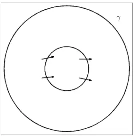
Definition 2.2.. LetM, N ⊂Rⁿbe open connected sets. The dynamical systemsϕ:T× M →M andψ :T×N →N are calledC^kequivalent, (fork = 0topologically equivalent), if there exists a C^k-diffeomorphismh:M →N (fork = 0a homeomorphism), that maps orbits onto each other by preserving the direction of time. This is shown in Figure 2.1.

In more detail, this means that there exists a continuous function a : T×M → T, for which t7→a(t, p) is a strictly increasing bijection and for all t∈T and p∈M we have

h ϕ(t, p)

=ψ a(t, p), h(p) .

One can get different notions of equivalence by choosing functions a and h having special properties. The above general equivalence will be referred to as equivalence of type 1. Now we define important special cases that will be called equivalences of type 2, 3 and 4.

Definition 2.3.. The dynamical systems ϕ and ψ are called C^k flow equivalent (equivalence of type 2), if in the general definition above, the function a does not depend on p, that is there exists a strictly increasing bijection b : T →T, for which a(t, p) = b(t) for all p∈M. Thus the reparametrization of time is the same on each orbit.

Definition 2.4.. The dynamical systems ϕ and ψ are called C^k conjugate (equivalence of type 3), if in the general definition above a(t, p) = t for all t ∈ T and p ∈ M. Thus there is no reparametrization of time along the orbits. In this case the condition of equivalence takes the form

h ϕ(t, p)

=ψ t, h(p) .

Definition 2.5.. The dynamical systems ϕ and ψ are called C^k orbitally equivalent (equivalence of type 4), if in the general definition above M = N and h = id, that is the orbits are the same in the two systems and time is reparametrized.

The definitions above obviously imply that the different types of equivalences are related in the following way.

(14)

Figure 2.1: The orbits of topologically equivalent systems can be taken onto each other by a homeomorphism.

Proposition 2.1. 1. If the dynamical systems ϕ and ψ are C^k conjugate, then they are C^k flow equivalent.

2. If the dynamical systems ϕ and ψ are C^k flow equivalent, then they are C^k equivalent.

3. If the dynamical systems ϕ and ψ are orbitally equivalent, then they are C^k equivalent.

Summarizing, the equivalences follows from each other as follows 3⇒2⇒1, 4⇒1.

2.1.1 Discrete time dynamical systems

First we show that for discrete time dynamical systems there is only one notion of equivalence, as it is formulated in the proposition below.

Letϕ:Z×M →M andψ :Z×N →N be discrete time dynamical systems. Let us define function f and g by f(p) = ϕ(1, p) and g(p) = ψ(1, p). Then the definition of a dynamical system simply implies thatϕ(n, p) =fⁿ(p) andψ(n, p) = gⁿ(p), wherefⁿand gⁿ denote the composition of the functions with themselvesn times, fⁿ =f ◦f ◦. . .◦f and similarly for g.

(15)

Proposition 2.2. The statements below are equivalent.

1. The dynamical systems ϕ and ψ are C^k conjugate.

2. The dynamical systems ϕ and ψ are C^k flow equivalent.

3. The dynamical systems ϕ and ψ are C^k equivalent.

4. There exists a C^k-diffeomorphism h:M →N, for which h◦f =g◦h.

Proof. According to the previous proposition the first three statements follow from each other from top to the bottom. First we prove that the last statement implies the first.

Then it will be shown that the third statement implies the last.

Using that h◦f =g◦h one obtains h◦f² =h◦f◦f =

h◦f|{z}=g◦h

g◦h◦f =

h◦f=g◦h|{z}

g ◦g◦h =g²◦h.

Similarly, the condition h ◦ fⁿ⁻¹ = gⁿ⁻¹ ◦ h implies h fⁿ(p)

= gⁿ h(p)

, that is h ϕ(n, p)

= ψ n, h(p)

holds for all n and p that is exactly the C^k conjugacy of the dynamical systems ϕand ψ.

Let us assume now that the dynamical systems ϕ and ψ are C^k equivalent. Let us observe first that if r : Z → Z is a strictly increasing bijection, then there exists k ∈ Z, such that r(n) = n +k for all n ∈ Z. Namely, strict monotonicity implies r(n+ 1) > r(n), while since r is a bijection there is no integer between r(n+ 1) and r(n), thus r(n+ 1) = r(n) + 1. Then introducing k = r(0) we get by induction that r(n) = n+k. Thus for the function a in the definition of C^k equivalence holds that for all p ∈ M there exists an integer k_p ∈ Z, for which a(n, p) = n+k_p. Thus the C^k equivalence of ϕand ψ means that for all n ∈Zand for all p∈M

h ϕ(n, p)

=ψ n+k_p, h(p) holds, that is

h fⁿ(p)

=g^n+k^p h(p) .

Applying this relation for n = 0 we get h(p) = g^k^p(h(p)). Then applying with n = 1 equation

h f(p)

=g^1+k^p h(p)

=g g^k^p h(p)

=g h(p) follows, that yields the desired statement.

Proposition 2.3. The dynamical systems ϕ and ψ are orbitally equivalent if and only if they are equal.

(16)

Proof. If the two dynamical systems are equal, then they are obviously orbitally equivalent. In the opposite way, if they are orbitally equivalent, then they are C^k equivalent, hence according to the previous proposition h◦f =g◦h. On the other hand,h=id implying f =g, thus ϕ(n, p) =ψ(n, p) for all n ∈Z, which means that the two dynamical systems are equal.

Definition 2.6.. In the case of discrete time dynamical systems, i.e. when T =Z, the functions f and g and the corresponding dynamical systems are called C^k conjugate if there exists a C^k-diffeomorphism h:M →N, for which h◦f =g◦h.

Remark 2.1. In this case the functions f and g can be transformed to each other by a coordinate transformation.

Proposition 2.4. In the case k >1, if f and g are C^k conjugate and p∈M is a fixed point of the map f (in this case h(p) is obviously a fixed point of g), then the matrices f⁰(p) and g⁰(h(p)) are similar.

Proof. Differentiating the equation h◦f =g◦h at the point pand using that f(p) =p and g(h(p)) = h(p) we get h⁰(p)f⁰(p) = g⁰(h(p))h⁰(p). This can be multiplied by the inverse of the matrix h⁰(p) (the existence of which follows from the fact that h is a C^k-diffeomorphism) yielding that the matrices f⁰(p) andg⁰(h(p)) are similar.

Remark 2.2. According to the above proposition C^k conjugacy (for k ≥1) yields finer classification than we need. Namely, the maps f(x) = 2xand g(x) = 3x are notC^k conjugate (since the eigenvalues of their derivatives are different), while the phase portraits of the corresponding dynamical systems x_n+1 = 2x_n and x_n+1 = 3x_n are considered to be the same (all trajectories tend to infinity). We will see that they are C⁰ conjugate, hence the above proposition is not true for k = 0.

2.1.2 Continuous time dynamical systems

Let us turn now to the study of continuous time dynamical systems, i.e. let T=R and let ϕ:R×M → M and ψ :R×N →N be continuous time dynamical systems. Then there are continuously differentiable functions f : M → Rⁿ and g : N → Rⁿ, such that the solutions of ˙x=f(x) are given by ϕand those of ˙y=g(y) are given by ψ.

Proposition 2.5. 1. Let k ≥ 1. Then the dynamical systems ϕ and ψ are C^k conjugate if and only if there exists a C^k diffeomorphism h : M → N C^k, for which h⁰·f =g◦h holds.

2. Assume that the function t7→a(t, p) is differentiable. Then the dynamical systems ϕ and ψ are orbitally equivalent if and only if there exists a continuous function v :M →R⁺, for which g =f ·v.

(17)

3. In Proposition 2.1 the converse of the implications are not true.

Proof. 1. First, let us assume that the dynamical systems ϕ and ψ are C^k conjugate.

Then there exists a C^k diffeomorphism h : M → N, for which h(ϕ(t, p)) = ψ(t, h(p)).

Differentiating this equation with respect to t we get h⁰(ϕ(t, p))·ϕ(t, p) = ˙˙ ψ(t, h(p)).

Since ϕ is the solution of ˙x=f(x) andψ is the solution of ˙y=g(y), we have h⁰(ϕ(t, p))·f(ϕ(t, p)) =g(ψ(t, h(p))).

Applying this for t = 0 yields

h⁰(ϕ(0, p))·f(ϕ(0, p)) =g(ψ(0, h(p))),

that is h⁰(p)·f(p) = g(h(p)). Thus the first implication is proved. Let us assume now that there exists a C^k-diffeomorphism h:M →N, for whichh⁰·f =g◦hholds. Let us define ψ^∗(t, q) :=h(ϕ(t, h⁻¹(q))) and then prove that this function is the solution of the differential equation ˙y=g(y). Then by the uniqueness of the solutionψ^∗ =ψ is implied, which yields the desired statement since substituting q =h(p) into the definition of ψ^∗ we get that ϕ and ψ are C^k conjugate. On one hand, ψ^∗(0, q) := h(ϕ(0, h⁻¹(q))) = q holds, on the other hand,

ψ˙^∗(t, q) =h⁰(ϕ(t, h⁻¹(q)))·ϕ(t, h˙ ⁻¹(q))

=h⁰(h⁻¹(ψ^∗(t, q)))·f(h⁻¹(ψ^∗(t, q))) =g(ψ^∗(t, q)), which proves the statement.

2. First, let us assume that the dynamical systems ϕ and ψ are orbitally equivalent. Then ϕ(t, p) = ψ(a(t, p), p), the derivative of which with respect to t is ˙ϕ(t, p) = ψ˙(a(t, p), p)·a(t, p). Since˙ ϕis the solution of ˙x=f(x) andψ is the solution of ˙y =g(y), we have f(ϕ(t, p)) =g(ψ(a(t, p)), p)). Applying this for t= 0 yields f(p) =g(p)·a(0, p),˙ which proves the statement by introducing the functionv(p) = ˙a(0, p). Assume now that there exists a functionv :M →R⁺, for whichg =f·v. Letp∈Rⁿand letx(t) = ϕ(t, p).

Introducing

b(t) = Z t

0

1 v(x(s))ds,

we have ˙b(t) = 1/v(x(t)) >0, hence the function b is invertible, the inverse is denoted by a=b⁻¹. (This function depends also on p, hence it is reasonable to use the notation a(t, p) =b⁻¹(t).) Lety(t) =x(a(t, p)), then

˙

y(t) = ˙x(a(t, p)) ˙a(t, p) = f(x(a(t, p))) 1

b(a(t, p))˙ =f(y(t))v(y(t)) =g(y(t)).

Hence y is the solution of the differential equation ˙y(t) =g(y(t)) and satisfies the initial condition y(0) = p, therefore y(t) = ψ(t, p). Thus using the definition y(t) = x(a(t, p)) we get the relation ψ(t, p) =ϕ(a(t, p), p) that was to be proved.

3. In order to prove this statement we show counterexamples.

(18)

(i) Let us introduce the matrices A=

0 1

−1 0

and B =

0 2

−2 0

. Then the phase portraits of the differential equations ˙x=Ax and ˙y=By are the same, since both of them are centers, however, the periods of the solutions in these two systems are different. Hence in order to map the orbits of the two systems onto each other time reparametrisation is needed. This means that the two systems are C^k flow- equivalent, however, they are not C^k conjugate.

(ii) Assume that bothϕand ψhas a pair of periodic orbits and the ratio of the periods is different in the two systems. Then they are not C^kflow-equivalent, but they can be C^k equivalent.

(iii) LetA=

1 0 0 −1

and B =

1 0 0 −2

. Then both ˙x=Axand ˙y=By determines a saddle point, that is they areC⁰ equivalent, however their orbits are not identical, hence they are not orbitally equivalent.

2.2 C

^k

classification of linear systems

In this section we classify continuous time linear systems of the form ˙x=Axand discrete time linear systems of the formx_n+1 =Ax_naccording to equivalence relations introduced in the previous section. Let us introduce the spaces

L(Rⁿ) ={A:Rⁿ →Rⁿ linear mapping}

and

GL(Rⁿ) = {A∈L(Rⁿ) : detA6= 0}

for the continuous and for the discrete time cases. If A ∈ L(Rⁿ), then the matrix A is considered to be the right hand side of the linear differential equation ˙x = Ax, while A ∈ GL(Rⁿ) is considered to be a linear map determining the discrete time system x_n+1 = Ax_n. Thus the space L(Rⁿ) represents continuous time and GL(Rⁿ) represents discrete time linear systems. In the linear case the dynamical system can be explicitly given in terms of the matrix. If A ∈ L(Rⁿ), then the dynamical system determined by A (that is the solution of the differential equation ˙x = Ax) is ϕ(t, p) = e^Atp. If A ∈ GL(Rⁿ), then the dynamical system generated by A (that is the solution of the recursion x_n+1 =Ax_n) isψ(n, p) = Aⁿp. In the following the equivalence of the matrices will be meant as the equivalence of the corresponding dynamical systems. Moreover, we will use the notion below.

Definition 2.7.. The matrices A and B are called linearly equivalent, if there exist α >0 and an invertible matrix P, for which A=αP BP⁻¹ holds.

(19)

Proposition 2.6. Let T=R and k≥1.

1. The matrices A, B ∈L(Rⁿ) are C^k conjugate, if and only if they are similar.

2. The matrices A, B ∈ L(Rⁿ) are C^k equivalent, if and only if they are linearly equivalent.

Proof. 1. Assume that the matrices AandB areC^k conjugate, that is there exists aC^k- diffeomorphism h : Rⁿ → Rⁿ, such that h(ϕ(t, p)) = ψ(t, h(p)), i.e. h(e^Atp) = e^Bth(p).

Differentiating this equation with respect to p we get h⁰(eÂtp)·eÂt = e^Bth⁰(p), then substitutingp= 0 yieldsh⁰(0)eÂt =e^Bt·h⁰(0). Differentiating now with respect totleads toh⁰(0)eÂt·A=e^Bt·B·h⁰(0), from which by substitutingt= 0 we geth⁰(0)A =B·h⁰(0).

The matrix h⁰(0) is invertible, because h is a diffeomorphism, hence multiplying the equation by this inverse we arrive to A = h⁰(0)⁻¹Bh⁰(0), i.e. the matrices A and B are similar. Assume now, that the matrices A and B are similar, that is there exists an invertible matrix P, for which A = P⁻¹BP. Then the linear function h(p) = P p is a C^k-diffeomorphism taking the orbits onto each other by preserving time, namely P e^Atp=P e^P⁻¹^{BP t}p=e^BtP p.

2. Assume that the matrices A and B are C^k equivalent, that is there exists a C^k-diffeomorphism h : Rⁿ → Rⁿ C^k and a differentiable function a : R ×Rⁿ → R, such that h(ϕ(t, p)) = ψ(a(t, p), h(p)), that is h(e^Atp) = e^Ba(t,p)h(p). Differentiating this equation with respect to p and substituting p = 0 yields h⁰(0)e^At = e^Ba(t,0) ·h⁰(0).

Differentiating now with respect to t we get h⁰(0)e^At·A=e^Ba(t,0) ·Ba(t,˙ 0)·h⁰(0), from which by substituting t = 0 we obtain h⁰(0)A = Ba(0,˙ 0)·h⁰(0). The matrix h⁰(0) is invertible, because his a diffeomorphism, hence multiplying the equation by this inverse and introducing α= ˙a(0,0) we arrive to A=αh⁰(0)⁻¹Bh⁰(0), i.e. the matrices A and B are linearly equivalent. Assume now, that the matrices A and B are linearly equivalent, that is there exists an invertible matrix P and α > 0, for which A = αP⁻¹BP. Then the linear function h(p) =P p is a C^k-diffeomorphism taking the orbits onto each other with time reparametrisation a(t, p) =αt, namelyP e^Atp=P e^αP⁻¹^{BP t}p=e^BαtP p.

Remark 2.3. According to the above proposition the classification given byC^k conjugacy and equivalence is too fine when k ≥1. Namely, the matrices A=

−1 0 0 −1

and B = −1 0

0 −2

are neither C^k conjugate nor C^k equivalent, however, they both determine a stable node, hence we do not want them to be in different classes since the behaviour of the trajectories is the same in the two systems. We will see that this cannot happen to matrices that are C⁰ conjugate, that is the above proposition does not hold for k = 0.

Proposition 2.7. Let T =Z and k ≥ 1. The matrices A, B ∈ GL(Rⁿ) are C^k conjugate, if and only if they are similar.

(20)

Proof. Assume that the matrices A and B are C^k conjugate, that is there exists a C^k-diffeomorphism h : Rⁿ → Rⁿ, for which h(Ap) = Bh(p). Differentiating this equation with respect to p yields h⁰(Ap)A = Bh⁰(p), then substituting p = 0 we get h⁰(0)A = Bh⁰(0). The matrix h⁰(0) is invertible, because h is a diffeomorphism, hence multiplying the equation by this inverse A =h⁰(0)⁻¹Bh⁰(0), that is the matrices A and B are similar. Assume now, that the matrices A and B are similar, that is there exists an invertible matrix P, for which A=P⁻¹BP. Then the linear function h(p) =P p is a C^k-diffeomorphism taking the orbits onto each other, namely P Ap=BP p.

2.3 C

⁰

classification of linear systems

In this section the following questions will be studied.

1. How can it be decided if two matrices A, B ∈ L(Rⁿ) are C⁰ equivalent or C⁰ conjugate?

2. How can it be decided if two matrices A, B ∈GL(Rⁿ) are C⁰ conjugate?

First, we answer these questions in one dimension.

2.3.1 Continuous time case in n = 1 dimension

Let us consider the differential equation ˙x =ax. If a <0, then the origin is asymptot- ically stable, i.e. all solutions tend to the origin as t → ∞. If a > 0, then the origin is unstable, i.e. all solutions tend to infinity as t → ∞. If a = 0, then every point is a steady state. These phase portraits are shown in Figure 2.2 for positive, zero and negative values of a. Thus the linear equations ˙x =ax and ˙y = by, in which a, b ∈ R, are C⁰ equivalent if and only if sgn a = sgn b. (The homeomorphism can be taken as the identity in this case.)

2.3.2 Discrete time case in n = 1 dimension

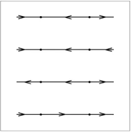
Let us consider the discrete time dynamical system given by the recursion x_n+1 = ax_n for different values of a ∈ R\ {0}. We note that the set GL(R) can be identified with the set R\ {0}. Since this recursion defines a geometric sequence, the behaviour of the trajectories can easily be determined. C⁰ equivalence divides GL(R) into the following six classes.

1. If a >1, then for a positive initial conditionx₀ the sequence is strictly increasing, hence 0 is an unstable fixed point.

2. If a= 1, then every point is a fixed point.

(21)

Figure 2.2: Three classes of continuous time linear equations in one dimension.

3. If 0 < a < 1, then 0 is a stable fixed point, every solution converges to zero monotonically.

4. If −1 < a < 0, then 0 is a stable fixed point, every solution converges to zero as an alternating sequence. Hence this is not conjugate to the previous case since a homeomorphism takes a segment onto a segment.

5. If a=−1, then the solution is an alternating sequence.

6. If a < −1, then 0 is an unstable fixed point, however, the sequence is alternating, hence this case is not conjugate to the case a >1.

For the rigorous justification of the above classification we determine the homeomorphism yielding the conjugacy.

To given numbers a, b∈R\ {0} we look for a homeomorphism h:R→R, for which h(ax) =bh(x) holds for all x. The homeomorphism h can be looked for in the form

h(x) =

x^α if x >0

−(−x)^α if x <0

If a, b > 0 and x > 0, then from equation h(ax) = bh(x) we get a^αx^α = bx^α, hence a^α =b, i.e. α= ^ln_lna^b. The function h is a homeomorphism, if α > 0, that holds, if a and b lie on the same side of 1. Thus if a, b > 1, then the two equations are C⁰ conjugate,

(22)

and similarly, if a, b ∈ (0,1), then the two equations are also C⁰ conjugate. (It can be seen easily that the equation h(ax) = bh(x) holds also for negative values of x.) One can prove similarly, that if a, b < −1 or if a, b ∈ (−1,0), then the two equations are C⁰ conjugate. Thus using the above homeomorphism h(x) = |x|^αsgn(x) we can prove that C⁰ conjugacy divides GL(R) at most into six classes. It is easy to show that there are in fact six classes, that is taking two elements from different classes they are not C⁰ conjugate, i.e. it cannot be given a homeomorphism, for which h(ax) = bh(x) holds for all x.

2.3.3 Continuous time case in n dimension

Let us consider the system of linear differential equations ˙x =Ax, where A is an n×n matrix. The C⁰ classification is based on the stable, unstable and center subspaces, the definitions and properties of which are presented first. Let us denote byλ₁, λ₂, . . . , λ_nthe eigenvalues of the matrix (counting with multiplicity). Let us denote by u₁, u₂, . . . , u_n the basis in Rⁿ that yields the real Jordan canonical form of the matrix. The general method for determining this basis would need sophisticated preparation, however, in the most important special cases the basis can easily be given as follows. If the eigenvalues are real and different, then the basis vectors are the corresponding eigenvectors. If there are complex conjugate pairs of eigenvalues, then the real and imaginary part of the corresponding complex eigenvector should be put in the basis. If there are eigenvalues with multiplicity higher than 1 and lower dimensional eigenspace, then generalised eigenvectors have to be put into the basis. For example, if λ is a double eigenvalue with a one dimensional eigenspace, then the generalised eigenvector v is determined by the equation Av =λv+u, where u is the unique eigenvector. We note, that in this case v is a vector that is linearly independent from u and satisfying (A−λI)²v = 0, namely (A−λI)²v = (A−λI)u= 0. Using this basis the stable, unstable and center subspaces can be defined as follows.

Definition 2.8.. Let {u₁, . . . , u_n} ⊂Rⁿ be the basis determining the real Jordan canonical form of the matrix A. Let λ_k be the eigenvalue corresponding to u_k. The subspaces

E_s(A) =h{u_k :Reλ_k<0}i, E_u(A) =h{u_k :Reλ_k >0}i, Ec(A) =h{uk :Reλk= 0}i

are called the stable, unstable and center subspaces of the linear system x˙ = Ax. (h·i denotes the subspace spanned by the vectors given between the brackets.)

The most important properties of these subspaces can be summarised as follows.

Theorem 2.9.. The subspaces E_s(A), E_u(A), E_c(A) have the following properties.

(23)

1. E_s(A)⊕E_u(A)⊕E_c(A) =Rⁿ

2. They are invariant under A(that is A(E_i(A))⊂E_i(A), i=s, u, c), and under e^At. 3. For all p∈E_s(A) we have e^Atp→0, if t→+∞, moreover, there exists K, α >0,

for which |e^Atp| ≤Ke^−αt|p|, if t≥0.

4. For all p∈E_u(A) we have e^Atp→0, ha t → −∞, moreover, there exists L, β > 0, for which |e^Atp| ≤Le^βt|p|, if t≤0.

The invariant subspaces can be shown easily for the matrixA=

1 0 0 −1

determining a saddle point. Then the eigenvalues of the matrix are 1 and −1, the corresponding eigenvectors are (1,0)^T and (0,1)^T. Hence the stable subspace is the vertical and the unstable subspace is the horizontal coordinate axis, as it is shown in Figure 2.3.

Figure 2.3: The stable and unstable subspaces for a saddle point.

The dimensions of the stable, unstable and center subspaces will play an important role in the C⁰ classification of linear systems. First, we introduce notations for the dimensions of these invariant subspaces.

Definition 2.10.. Lets(A) = dim(E_s(A)), u(A) = dim(E_u(A))andc(A) = dim(E_c(A)) denote the dimensions of the stable, unstable and center subspaces of a matrix A, respectively.

The spectrum, i.e. the set of eigenvalues of the matrix A will be denoted by σ(A).

The following set of matrices is important from the classification point of view. The elements of

EL(Rⁿ) ={A ∈L(Rⁿ) :Reλ6= 0, ∀λ ∈σ(A)},

(24)

are called hyperbolic matrices in the continuous time case.

First, these hyperbolic systems will be classified according to C⁰-conjugacy. In order to carry out that we will need the Lemma below.

Lemma 2.11.. 1. If s(A) = n, then the matrices A and −I are C⁰ conjugate.

2. If u(A) =n, then the matrices A and I are C⁰ conjugate.

Proof. We prove only the first statement. The second one follows from the first one if it is applied to the matrix −A. The proof is divided into four steps.

a. The solution of the differential equation ˙x= Ax starting from the point p is x(t) = e^Atp, the solution of the differential equation ˙y = −y starting from the same point is y(t) = e^−tp. According to the theorem about quadratic Lyapunov functions there exists a positive definite symmetric matrix B ∈ R^n×n, such that for the corresponding quadratic form Q_B(p) =hBp, pi it holds that L_AQ_B is negative definite. We recall that (L_AQ_B)(p) =hQ⁰_B(p), Api. The level set of the quadratic formQ_B belonging to the value 1 is denoted by S :={p∈Rⁿ :Q_B(p) = 1}.

b. Any non-trivial trajectory of the differential equation ˙x = Ax intersects the set S exactly once, that is for any point p∈ Rⁿ\ {0} there exists a unique number τ(p)∈R, such that eÂτ(p)p ∈S. Namely, the function V^∗(t) = Q_B(eÂtp) is strictly decreasing for any p ∈ Rⁿ\ {0} and lim+∞V^∗ = 0, lim−∞V^∗ = +∞. The function τ : Rⁿ\ {0} → R is continuous (by the continuous dependence of the solution on the initial condition), moreover τ(eÂtp) = τ(p)−t.

c. Now, the homeomorphism taking the orbits of the two systems onto each other can be given as follows

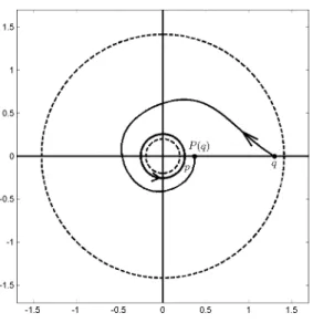
h(p) :=e^(A+I)τ(p)p, if p6= 0, and h(0) = 0.

This definition can be explained as follows. The mapping takes the point first to the set S along the orbit of ˙x = Ax. The time for taking p to S is denoted by τ(p). Then it takes this point back along the orbit of ˙y=−y with the same time, see Figure2.4.

d. In this last step, it is shown that h is a homeomorphism and maps orbits to orbits.

The latter means that h(e^Atp) = e^−th(p). This is obvious for p = 0, otherwise, i.e. for p6= 0 we have

h(eÂtp) =e^(A+I)τ(eÂt^p)eÂtp=e(A+I)(τ(p)−t)eÂtp=e^(A+I)τ(p)e^−tp=e^−th(p).

Thus it remains to prove that h is a homeomorphism. SinceL−IQ_B =Q−2B is negative definite, the orbits of ˙y = −y intersect the set S exactly once, hence h is bijective (its inverse can be given in a similar form). Because of the continuity of the function τ the functions h and h⁻¹ are continuous at every point except 0. Thus the only thing that remained to be proved is the continuity of h at zero. In order to that we show that

limp→0e^τ(p)e^Aτ^(p)p= 0.

(25)

Since e^Aτ(p)p∈ S and S is bounded, it is enough to prove that lim_p→0τ(p) =−∞, that is for any positive number T there exists δ >0, such that it takes at least time T to get from the set S to the ball B_δ(0) along a trajectory of ˙x=Ax. In order to that we prove that there existsγ <0, such that for all pointsp∈S we havee^γt ≤Q_B(e^Atp), that is the convergence of the solutions to zero can be estimated also from below. (Then obviously

|eÂtp|can also be estimated from below.) LetCbe the negative definite matrix, for which LAQB = QC. The negative definiteness of C and the positive definiteness of B imply that there exist α < 0 and β > 0, such that Q_C(p) ≥ α|p|² and Q_B(p) ≥ β|p|² for all p ∈ Rⁿ. Let V^∗(t) := Q_B(eÂtp) (for an arbitrary point p∈ S), then ˙V^∗(t) = Q_C(eÂtp), hence ˙V^∗(t)QB(eÂtp) = V^∗(t)QC(eÂtp) implying βV˙^∗(t) ≥ αV^∗(t). Let γ := ^α_β, then Gronwall’s lemma implies that V^∗(t)≥e^γt, that we wanted to prove.

Figure 2.4: The homeomorphism h taking the orbits of ˙x=Ax to the orbits of ˙y=−y.

Using this lemma it is easy to prove the theorem below about the classification of hyperbolic linear systems.

Theorem 2.12.. The hyperbolic matrices A, B ∈ EL(Rⁿ) are C⁰ conjugate, and at the same time C⁰ equivalent, if and only if s(A) = s(B). (In this case, obviously, u(A) = u(B) holds as well, since the center subspaces are zero dimensional.)

The C⁰ classification is based on the strong theorem below, the proof of which is beyond the framework of this lecture notes.

(26)

Theorem 2.13. (Kuiper). Let A, B ∈ L(Rⁿ) be matrices with c(A) = c(B) = n.

These are C⁰ equivalent, if and only if they are linearly equivalent.

The full classification below follows easily from the two theorems above.

Theorem 2.14.. The matrices A, B ∈ L(Rⁿ) are C⁰ equivalent, if and only if s(A) = s(B), u(A) = u(B) and their restriction to their center subspaces are linearly equivalent (i.e. A|Ec and B|Ec are linearly equivalent).

Example 2.1. The space of two-dimensional linear systems, that is the space L(R²) is divided into 8 classes according to C⁰ equivalence. We list the classes according to the dimension of the center subspaces of the corresponding matrices.

1. If c(A) = 0, then the dimension of the stable subspace can be 0, 1 or 2, hence there are three classes. The simplest representants of these classes are

A= 1 0

0 1

, A=

1 0 0 −1

, A =

−1 0 0 −1

,

corresponding to the unstable node (or focus), saddle and stable node (or focus), respectively. (We recall that the node and focus are C⁰ conjugate.) The phase portraits belonging to these cases are shown in Figures 2.5, 2.6 and 2.7.

Figure 2.5: Unstable node.

2. If c(A) = 1, then the dimension of the stable subspace can be 0 or 1, hence there are two classes. The simplest representants of these classes are

A= 1 0

0 0

, A=

−1 0

0 0

.

The phase portraits belonging to these cases are shown in Figures 2.8 and 2.9.

(27)

Figure 2.6: Saddle point.

Figure 2.7: Stable node.

3. If c(A) = 2, then the classes are determined by linear equivalence. If zero is a double eigenvalue, then we get two classes, and all matrices having pure imaginary eigenvalues are linearly equivalent to each other, hence they form a single class.

Hence there are 3 classes altogether, simple representants of which are A =

0 0 0 0

, A= 0 1

0 0

, A =

0 −1

1 0

.

The last one is the center. The phase portraits belonging to these cases are shown in Figures 2.10, 2.11 and 2.12.

(28)

Figure 2.8: Infinitely many unstable equilibria.

Figure 2.9: Infinitely many stable equilibria.

It can be shown similarly that the space L(R³) of 3-dimensional linear systems is divided into 17 classes according to C⁰ equivalence.

The spaceL(R⁴) of 4-dimensional linear systems is divided into infinitely many classes according to C⁰ equivalence, that is there are infinitely many different 4-dimensional linear phase portraits.

(29)

Figure 2.10: Every point is an equilibrium.

Figure 2.11: Degenerate equilibria lying along a line.

2.3.4 Discrete time case in n dimension

Consider the system defined by the linear recursion xk+1 = Axk, where A is an n×n matrix. The C⁰ classification uses again the stable, unstable and center subspaces, that will be defined first, for discrete time systems. Let us denote the eigenvalues of the matrix with multiplicity by λ1, λ2, . . . , λn. Let u1, u2, . . . , un denote that basis in Rⁿ in which the matrix takes it Jordan canonical form. Using this basis the stable, unstable and center subspaces can be defined as follows.

Definition 2.15.. Let {u1, . . . , un} ⊂Rⁿ be the above basis and let λk be the eigenvalue

(30)

Figure 2.12: Center.

corresponding to uk (note that uk may not be an eigenvector). The subspaces E_s(A) =h{u_k :|λ_k|<1}i, E_u(A) =h{u_k :|λ_k|>1}i,

E_c(A) =h{u_k :|λ_k|= 1}i

are called the stable, unstable and center subspaces belonging to the matrix A∈GL(Rⁿ).

(The notation h·i denotes the subspace spanned by the vectors between the brackets.) The most important properties of these subspaces are summarised in the following theorem.

Theorem 2.16.. The subspaces E_s(A), E_u(A), E_c(A) have the following properties.

1. E_s(A)⊕E_u(A)⊕E_c(A) =Rⁿ

2. They are invariant under A (that is A(E_i(A))⊂E_i(A), i=s, u, c).

3. For any p∈Es(A) we have Aⁿp→0, if n →+∞.

4. For any p∈E_u(A) we have A⁻ⁿp→0, if n→+∞.

The dimensions of the stable, unstable and center subspaces will play an important role in the C⁰ classification of linear systems. First, we introduce notations for the dimensions of these invariant subspaces.

Definition 2.17.. Lets(A) = dim(E_s(A)), u(A) = dim(E_u(A))andc(A) = dim(E_c(A)) denote the dimensions of the stable, unstable and center subspaces of a matrix A, respectively.

(31)

The following set of matrices is important from the classification point of view. The elements of

HL(R) ={A∈GL(Rⁿ) :|λ| 6= 1 ∀λ∈σ(A)}, are called hyperbolic matrices in the discrete time case.

In the discrete time case only the hyperbolic systems will be classified according to C⁰-conjugacy. In order to carry out that we will need the Lemma below.

Lemma 2.18.. Let the hyperbolic matrices A, B ∈ HL(Rⁿ) be C⁰ conjugate, that is there exists a homeomorphism h : Rⁿ → Rⁿ, for which h(Ax) =Bh(x) for all x ∈ Rⁿ. Then the following statements hold.

1. h(0) = 0, 2. h E_s(A)

=E_s(B), that ishtakes the stable subspace to stable subspace; h E_u(A)

= E_u(B), that is h takes the unstable subspace to unstable subspace

3. s(A) =s(B), u(A) =u(B).

Proof. 1. Substituting x= 0 into equation h(Ax) =Bh(x) leads to h(0) =Bh(0). This implies that h(0) = 0, because the matrix B is hyperbolic, that is 1 is not an eigenvalue.

2. If x ∈ E_s(A), then Aⁿ → 0 as n → ∞, hence h(Aⁿx) = Bⁿh(x) implies that Bⁿh(x) tends also to zero. Therefore h(x) is in the stable subspace of B. Thus we showed that h E_s(A)

⊂ E_s(B). Using similar arguments for the function h⁻¹ we get that h⁻¹ E_s(A)

⊂ E_s(B) yielding E_s(B)⊂ h E_s(A)

. Since the two sets contain each other, they are equal h E_s(A)

=E_s(B).

3. Since there is a homeomorphism taking the subspaceE_s(A) to the subspaceE_s(B), their dimensions are equal, i.e. s(A) = s(B), implying also u(A) = u(B) since the dimensions of the center subspaces are zero.

In the case of continuous time linear systems we found that s(A) =s(B) is not only a necessary, but also a sufficient condition for the C⁰ conjugacy of two hyperbolic linear systems. Now we will investigate in the case of a one-dimensional and a two-dimensional example if this condition is sufficient or not for discrete time linear systems.

Example 2.2. Consider the one-dimensional linear equations given by the numbers (one-by-one matrices) A = ¹₂ and B = −¹₂. Both have one dimensional stable subspace, that is s(A) = s(B) = 1, since the orbits of both systems are formed by geometric sequences converging to zero. However, as it was shown in Section 2.3.2, these two equations are not C⁰ conjugate. It was proved there that C⁰ conjugacy divides the space GL(R) into six classes.

(32)

This example shows that s(A) = s(B) is not sufficient for the C⁰ conjugacy of the two equations. Despite of this seemingly negative result, it is worth to investigate the following two dimensional example, in order to get intuition for the classification of hyperbolic linear systems.

Example 2.3. Consider the two-by-two matrices A= ¹₂I and B =−¹₂I, where I is the unit matrix. The stable subspace is two-dimensional for both systems, that is s(A) = s(B) = 2, since their orbits are given by sequences converging to zero. We will show that these matrices are C⁰ conjugate. We are looking for a homeomorphism h : R² → R² satisfying h(¹₂x) = −¹₂h(x) for all x ∈ R². It will be given in such a way that circles centered at the origin remain invariant, they will be rotated by different angles depending on the radius of the circle. Let us start from the unit circle with radius one and definehas the identity map on this circle, i.e. h(x) =x is |x|= 1. Then equation h(¹₂x) =−¹₂h(x) defines h along the circle of radius1/2, namely h rotates this circle byπ, i.e. h(x) =−x is |x|= 1/2. In the annulus between the two circles the homeomorphism can be defined arbitrarily. Then equation h(¹₂x) = −¹₂h(x) defines h again in the annulus between the circles of radius 1/2 and 1/4. Once the function is known in this annulus the equation defines again its values in the annulus between the circles of radius 1/4 and 1/8. In a similar way, the values of h in the annulus between the circles of radius 1 and 2 are defined by the equation h(¹₂x) = −¹₂h(x) based on the values in the annulus determined by the circles of radius 1/2 and 1. It can be easily seen that the angle of rotation on the circle of radius 2^k has to be −kπ. Thus let the angle of rotation on the circle of radius r be −πlog₂(r). This ensures that the angle of rotation is a continuous function of the radius and for r = 2^k it is −kπ. This way the function h can be given explicitly on the whole plane as follows

h(x) = R(−πlog₂(|x|))x, where R(α) =

cosα sinα

−sinα cosα

This function is obviously bijective, since the circles centered at the origin are invariant and the map is bijective on these circles. Its continuity is also obvious except at the origin. The continuity at the origin can be proved by using the above formula, we omit here the details of the proof.

We note that in 3-dimension the matrices A = ¹₂I and B = −¹₂I, where I is the unit matrix of size 3 ×3, are not C⁰ conjugate. Thus we found that s(A) = s(B) is not a sufficient condition of C⁰ conjugacy. The sufficient condition is formulated in the following lemma that we do not prove here.

Lemma 2.19.. Assume that s(A) = s(B) = n (or u(A) = u(B) = n). Then A and B are C⁰ conjugate, if and only if sgndetA=sgndetB.

This lemma enables us to formulate the following necessary and sufficient condition for the C⁰ conjugacy of matrices.