DOI: 10.1556/606.2018.13.2.10 Vol. 13, No. 2, pp. 97–106 (2018) www.akademiai.com
EFFECT OF AERATION ON RESIDENCE TIME IN BIOLOGICAL WASTEWATER TREATMENT
Tamas KARCHES
Institute of Water Supply and Environmental Engineering, Faculty of Water Science National University of Public Service, Bajcsy-Zsilinszky u. 12-14, H-6500 Baja, Hungary
e-mail: Karches.Tamas@uni-nke.hu
Received 17 December 2017; accepted 4 February 2018
Abstract: Aerobic wastewater treatment requires extensive aeration, which primary function is to provide oxygen to the biomass responsible for degradation of wastewater constituents.
Besides the effective oxygen transfer efficiency aeration is responsible for fluid flow created by bubbles. In this research bubbles were released from plate diffusers and the impact on mixing were analyzed. Various aeration flow rates and initial bubble sizes were calculated. Residence time distributions in each scenario were compared applying numerical tracer study. Outcome of the calculations is that the aeration reduces the theoretical residence time significantly and therefore the traditional sizing methods needs to be revisit in wastewater treatment.
Keywords: Aeration, Hydrodynamics, Residence time distribution, Multiphase flow, Wastewater treatment
1. Introduction
In biological wastewater treatment the degradation of organic material and some processes in nutrient removal require aerobic conditions, namely, the presence of dissolved oxygen in water phase. Based on Henry’s law the amount of dissolved oxygen is proportional to the partial pressure of the oxygen in the gas phase. Since the biomass oxygen uptake rate is higher than the natural replacement of oxygen due to Henry’s law, an aeration system is to be applied, which provides high degree of oxygen transfer to water phase intensifying wastewater treatment. As a design criterion for an activated sludge process, where the biomass is in suspended form, the Dissolved Oxygen (DO) concentration is about 2-3.0 mg/l, but never falls under below 1.8 mg/l. Lower DO
concentrations (0.5-2.0 mg/l) produces sludge with poorer settling characteristics compared to higher DO concentrations [1] and advanced settling techniques [2] shall be applied to achieve satisfactory level of phase separation.
There are two common types of wastewater aeration: surface and subsurface aeration. A surface aerator employs blades rotating around a horizontal (e.g. Kessener brush) or vertical shaft. The aerators can be placed to certain location or they are floating on water surface. Air is entrained behind the blades and due to the turbulence created the oxygen transfer into the wastewater is enhanced [3]. The oxygen transfer efficiency is about 1.2 to 2.4 kg O2/kWh. Subsurface aeration applies mainly diffusers releasing bubbles at the bottom of the water body. The bubbles released start to rise due to buoyancy. During their movement oxygen transfer is observable through the gas- water interface. The efficiency of mass transfer relies on the area of the interface, therefore generally relatively small bubbles (fine bubbles) with the diameter of 1 to 3 mm is applied. The benefits of using fine bubbles over surface aeration are the uniform oxygenation, higher dissolution time of oxygen and better oxygen transfer efficiency, thus less energy demand [4].
Besides converting organic matter into biological cell mass, aeration has impact on hydrodynamics of the reactor [5]. The achievable mixing efficiency depends on the form of the biomass, which can be suspended or attached to carrier (fixed film process).
In activated sludge systems, where the biomass is suspended, mixing is primarily achieved by mechanical mixers, but aeration also has effect on reactor hydraulics. In attached growth processes high degree of mixing is required for the effective use of biomass within the reactor [6]. In this case mixing is not only responsible for homogenization, but also provides enough energy for the substrate to be transported through the biofilm layers. In this system the turbulent diffusion generated by the main flow shall overcome the thin laminar layer on the biofilm surface. Furthermore, depending on the roughness of the biofilm surface and flow conditions, the mass transfer into the biofilm relies on the eddy diffusion [7]. In 1994, Zhang and Bishop went further and realized that besides the increasing fluid stream-wise velocity, the increasing roughness of the biofilm surface and the increasing substrate loading rate would make the external mass transfer resistance decrease [8]. Since the aeration intensity has a direct effect on fluid flow, it also affects the biofilm kinetics. High aeration intensity would mean high detachment rate of the biofilm, low aeration intensity allows thick biofilm in the lack of shearing effect [9].
Aeration has impact on the reactor hydraulics, intensifies the mixing, increases turbulence [10]. If aeration intensity is examined in function with time, it can be
i) constant; or
ii) intermittent aeration.
Aerobic reactors are generally aerated by constant air flow or constant DO is applied.
Intermittent aeration is a combination of aerobic and anoxic conditions, with which nitrogen removal efficiency could be improved and control of N2O emission could be achieved [11].
Reactor hydrodynamics could take advantage of aeration by the so-called air lift effect. Airlift bioreactor is an alternative solution to stirred reactors; the cloud of bubbles is injected with a Reynolds number of 10 to 100. The micro bubbles are
generated by fluid oscillation. The oscillatory flow interrupts the air flow and limits the growth of the bubbles compared to fine bubble aeration. As a result of this process longer gas-liquid interaction time and higher interaction area is achieved [12], and thus the oxygen transfer efficiency is also enhanced [13]. As an effect of aeration induced flow, the circulation cell sizes is about four times higher than the depth of the reactor [14] if the boundaries allows to develop these eddies.
Residence time is a key parameter in designing technologies, since it could describe the unit processes without using the dimensions of the plants, basins or reactors. In wastewater treatment the detention time can be defined for water Hydraulic Residence Time (HRT) and for solid fraction Sludge Residence Time (SRT). HRT reflects to the detention of the water phase, whereas SRT is related to the biomass and substrate degradation and each biological process has an advisable SRT (e.g. at 12°C for organic matter removal it is 4-5 days and for nitrification it is 9-10 days). HRT can be determined by dividing the reactor volume with the discharge, which gives an average value for the entire reactor. SRT can be composed from HRT by applying solid concentrations as weighting factors; reactor volume shall be multiplied with Mixed Liquor Suspended Solid (MLSS) concentration and instead of wastewater discharge the wasted sludge with the multiplication of dry solid content is used. HRT and SRT are identical only if a lagoon system is in operation, but most of the cases the process contains sludge recirculation from secondary clarifier to biological reactor, which results that the HRT is significantly lower compared to SRT. Beside the SRT, other time-related parameters can be defined. One is sludge age, which is calculated as a ratio of the total solids in aeration tank to the weight of total solids in the aeration tank influent, the other is Mean Cell Residence Time (MCRT). The latter one is a combination of what is in the system and what exits as the effluent and as wasted sludge. At low effluent Total Suspended Solid (TSS) concentration the difference between SRT and MCRT is negligible. For process sizing SRT is the base, but it is in correlation with HRT. If the HRT decreases it is probable that SRT also decreases, giving the biomass less time for degradation the organic matter and nutrient removal, which may cause violation of effluent limits.
If inhomogeneity of sludge age within the reactor needs to be revealed, Residence Time Distribution (RTD) analysis could be an effective tool based on the idea that a given amount of tracer is introduced to the system and the effluent concentration, as a response function is measured in course of time. With the help of the normalized concentration curve small scale hydraulic phenomena can be estimated, e.g. as short circuiting, and dead-zones. This curve can be measured experimentally or compute using Computational Fluid Dynamic (CFD) techniques [15].
In this paper the effect of subsurface aeration on the residence time will be investigated, the methodology of the research is described in Section 2, the results are presented in Section 3 and the conclusions drawn are in Section 4.
2. Methodology
Conventional way to predict the aeration induced flow is performing numerical simulation, which solves the governing physical equations for the liquid as well as the
gaseous phase. Water is the primary phase; air is the secondary phase reflecting the volume fraction difference. Mass and momentum balance have to be solved in conservative form in order to describe the movement of bubbles. Widely used approach is finite volume method, which uses the integral form of the conservation equations as starting point and subdivides the reactor volume creating finite number of small control volumes (grid) [16]. The integral forms of conservation equations are solved in each control volume and flow variables are expressed in terms of the nodal values by interpolation [17]. From the numerous possible interpolation schemes the upwind scheme was used in this study. Advantage of this approach is that it never yields oscillatory solution, but it is exposed to numerical diffusion [18]. This modeling approach differs from finite element method widely applied in water network system modeling [19], concentrating global losses over the entire network. In this research more detailed micro scale model needs to be built.
Momentum and continuity equations are solved for each phase. In fluid-fluid flow each secondary phase is assumed to form droplets or bubbles. The exchange between the phases is based on the value of the fluid-fluid exchange coefficient. This coefficient depends on the drag function, which is based on the relative Reynolds number. General solution can be adapted by e.g. Schiller-Neumann approach [20]. In a liquid-gas multiphase flow there are two distinct regimes; the first one corresponds to low value of the secondary gaseous phase, where hydrodynamic interactions between bubbles are negligible and the second one with higher value, where the bubbles transfer significant amount of kinetic energy to the liquid phase [21].
One of the assumptions to describe two phase bubbly flow is that the phases are considered as continua and governed by partial differential equations of continuum mechanics [22]. The phases are separated by an interface, which can be defined as a surface in most of the cases. Direct Numeric Simulation (DNS) is restricted to model only small amount of bubbles due to its simulation cost; therefore it is inefficient in industrial applications. An effective simplification can be made if the variables are averaged over the entire simulation domain and in time, which lead to a Reynolds- Averaged Navier-Stokes (RANS) solution. Stress terms shall be defined in the momentum equations to express the turbulent stress and formulate a closure for Partial Differential Equations (PDEs). This closure is determined empirically, which is the calibration of the two-phase model. In this paper the calibrated parameters mentioned in literature are applied [23].
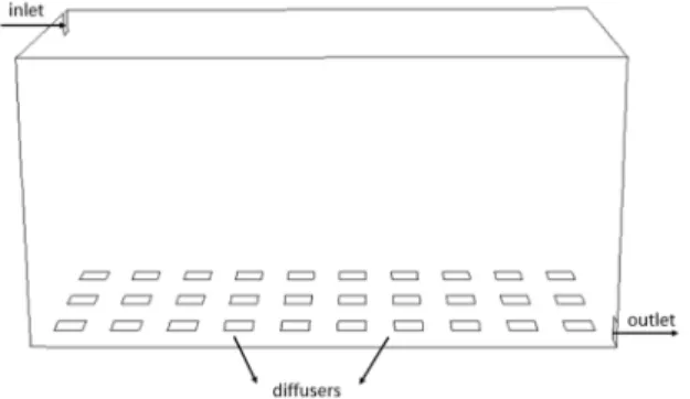
As a first step the simulation domain was built by drawing a rectangular model of an aerated reactor with 30 plate diffusers. The reactor has 12 m length, 6 m width and 6 m height. The diffusers are 0.2 from the bottom. The diffuser density is 0.15 m2 diffuser/m2 bottom surface. For spatial discretization 57660 cells, 62464 nodes and 177661 faces were created. Boundary conditions were the following: symmetry at the side of the model domain, since horizontal fluxes could happen through the interface. Zero-shear wall was set for the free surface boundary, applying a sink term to satisfy the continuity of air and taking into account the air amount leaving the system.
Wastewater was entered the reactor with 720 m3/d discharge, the theoretical residence time was 14.4 h. Model geometry can be seen on Fig. 1.
The above mentioned model configuration was used to determine the average actual residence time of wastewater in simulation domain. Model scenarios were defined with
1 m3/h and 4 m3/h aeration per diffusers and as a reference a model without aeration was also investigated.
Fig. 1. Model geometry, aerobic reactor applying plate diffusers
In addition, various bubble sizes from fine to coarse were also investigated. In each case the flow field was determined as a result of the calculation. With the knowledge of the velocity vector field at each simulation point, model tracers could be released: the path-lines of the tracer and the residence time distribution were determined following the Lagrangian approach as an evaluation method of the flow field [24]. By averaging the residence time of each single particle, an integral average value was gained. Besides the residence time, other flow parameters were also examined, average vertical and horizontal velocities. Complex mixing parameters (e.g. rotation, effective viscosity) were also calculated as a volume averaged integral and compared in each scenario.
Magnitude of each nodal velocity component value was used in the integration.
Effective viscosity in turbulent flow was able to reflect the effect of the micro fluctuation of velocity and result better mixing properties. Turbulent diffusion could be estimated as follows:
SC D eff
σ
= µ , (1)
where µeff is the effective turbulent viscosity and σSC is the Schmidt number, with a constant value of 0.7 [15].
3. Results and discussion
Numerical calculations were performed following the simulation processes described in Section 2, and the results were compared in these cases:
i) wastewater inflow, no aeration;
ii) wastewater inflow with 4 m3/h aeration per diffuser applying fine bubbles;
iii) wastewater inflow with 4 m3/h aeration per diffuser applying coarse bubbles;
iv) wastewater inflow with 1 m3/h aeration per diffuser applying fine bubbles.
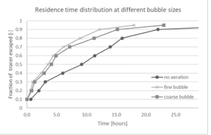
100 particles were injected at the inlet section to a pre-calculated flow field and the time spent of the particles in the reactor was tracked at the outflow section. The tracer had the same material properties as water had. Every single particle resided different time in the system, since the fate of the particles was conditioned by the turbulence, which has a stochastic property. Cumulative function was used to detect the fraction of the escaped tracer and it was drawn against time. Fig. 2 shows the distribution of residence/detention time of the tracer at different bubble sizes. In order to draw the baseline (flow without aeration) residence time distribution of scenario i) was also investigated.
Fig. 2. Residence time distribution at different bubble sizes
As Fig. 2 represents a small amount of tracer presented at the outlet boundary within 1 hour due to hydraulic shortcut in each scenario. Other part of the particles retained in the reactor more than two times of the theoretical average residence time, probably due to the presence of dead or stagnant zones. If there is no aeration, the actual residence time is 9.2 h, which is lower compared to the theoretical value (14.4 h). One reason is the presence of small scale hydraulic phenomena (shortcut, dead-zone); other is that the theoretical average residence time is a statistical average (first moment) in a confined water body at steady state conditions, not assuming the effect of turbulence. However, the turbulence could increase the dispersion and mixing rate. If high degree of mixing is present in our system the actual reactor model can be described by applying Completely Stirred Tank Reactor (CSTR) model. Fig. 2 also shows that particles appear continuously between in the first 25 hours, but as the time advances the rate of the particle discharging the reactor decreases.
Simulations were performed applying fine bubbles with diameter of 1 mm and coarse bubbles with diameter of 5 mm. It should be noted that this bubble size is an initial size, only valid at the releasing point of the diffusers; as the bubbles rise and/or collide the bubble diameters are growing. As a result of the simulations, water flow
induced by coarse bubbles has a slightly higher detention time; the average residence time is 3.5 h for fine bubble, 4.1 h for coarse bubble. Considerable difference can be observed between the scenarios, where aeration is applied or not. Based on Fig. 2 the HRT reduces by 60% if aeration is on. One possible explanation is that aeration gives surplus external energy, which induces water flow, increases mixing intensity and reduces the actual HRT.
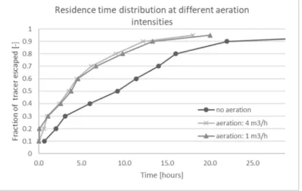
In Fig. 3 different aeration intensities were compared assuming fine bubble aeration.
Although the air flow rate is decreased by 75% it had no significant impact on residence time distribution as well as on the actual average detention time. In this reduced aeration reactor the calculated HRT was 3.8 h compared to 3.5 h in case of full aeration.
Fig. 3. Residence time distribution at different aeration intensities
For the calculation of the energy available for mixing the following terms shall be taken into account:
i) position of the inlet and outlet;
ii) aeration rate; and
iii) mechanical mixer performance, where the term iii) is not applicable in this case study.
The power utilized the mixing due to level difference between the inlet and outlet calculated as follows:
W 475
=
⋅
⋅
⋅
= g H Q
Pflow ρ , (2)
where ρ is the water density; g is the gravitational acceleration; H is the level difference between the inlet and outlet; Q is the wastewater discharge.
The mixing power of aeration is determined as follows:
0 ln p Q p
p
Paeration= a⋅ aeration⋅ diff , (3)
where pa is the atmospheric pressure; pdiff is the pressure at the diffuser level; Qaeration is the aeration volume flux. The aeration power is about 1500 W at 4 m3/h air flow rate and 375 W for 1 m3/h air flow rate respectively. It can be stated that with increasing power the HRT decreases, but the relation is non-linear. It should be noted that the aeration power is meaningful for the gas phase but flow induced at the wastewater side is not calculated. That explains why HRT differs between fine or coarse bubble aeration applying the same aeration power.
Flow properties in different scenarios were calculated as volume integral averages and summarized in Table I. Wastewater flow (as primary phase) velocities were divided to horizontal and vertical component, air velocities were averaged in three directions.
The effective viscosity due to the turbulence was also determined, and based on (1) the diffusion can be estimated.
Table I
Average flow properties at various scenarios
Scenario
Air flow rate per diffuser [m3/h]
Bubble type
Primary phase horizontal
velocity [m/s]
Primary phase vertical velocity
[m/s]
Primary phase effective viscosity [kg/(ms)]
Secondary phase velocity
[m/s]
i) no aeration no aeration 0.013 0.02 6.14 0
ii) 4 fine bubble 0.116 0.11 30.1 0.2
iii) 4 coarse
bubble
0.066 0.082 23.8 0.31
iv) 1 fine bubble 0.07 0.08 25.2 0.18
Table I shows that if there is no aeration the flow is rather vertical than horizontal (due to the position of the inlet and outlet boundaries), the effective viscosity has a 6.14 kg/(ms) background value. It increases sharply when aeration is on, the rising bubbles create turbulence. Fine bubbles have relatively higher surface area and it causes higher communication (momentum exchange) between gas and liquid phase leading higher velocities and effective viscosity, even though the air velocity is higher when coarse bubble aeration was applied. Table I states that the air velocity depends on the bubble size and weakly related to the air flow. For appropriate mixing and homogenization of substrate both the vertical and horizontal velocity components are important, and as the simulation results revealed if aeration is on, the velocity components are close, however the scenario without aeration showed vertical flow dominance.
4. Conclusion
Appropriate sizing of aerated basins in wastewater treatment is based on the knowledge of the actual average residence time. Determination of residence time distribution requires extensive knowledge of fluid flow, which is induced by subsurface aeration. In this research various aeration setups were investigated applying fluid flow simulations combined with numerical tracer study in order to reveal the actual flow and mixing conditions. With the help of the cumulative function of a tracer possible hydraulic shortcuts and stagnant zones could be detected. If coarse bubbles were in the system it had a slightly higher detention time compared to fine bubble induced flow, but overall consequence is that if external energy is introduced to the reactor and thus the diffusivity of the momentum is increased, the average HRT is decreased. The analysis also showed that the air velocity depends on the bubble size and weakly related to the air flow and air velocity does not correlate to the induced wastewater velocities. As the next step the residence time distribution will be investigated in reactors with various length/width ratios and diffuser density.
Acknowledgements
The work was created in commission of the National University of Public Service under the priority project KÖFOP-2.1.2-VEKOP-15-2016-00001 titled ‘Public Service Development Establishing Good Governance’ in István Egyed Postdoctoral Program.
References
[1] Wilén B. M., Balmér P. The effect of dissolved oxygen concentration on the structure, size and size distribution of activated sludge flocs, Water Research, Vol. 33, No. 2, 1999, pp. 391–400.
[2] Sándor D. B., Szabó A., Fleit E., Bakacsi Z., Zajzon G. PVA-PAA hydrogel micro-carrier for the improvement of phase separation efficiency of biomass in wastewater treatment.
Pollack Periodica, Vol. 12, No. 2, 2017, pp. 91–102.
[3] Cancino B. Design of high efficiency surface aerators: Part 2. Rating of surface aerator rotors, Aquacultural Engineering, Vol. 31, No. 1, 2004, pp. 99–115.
[4] McWhirter J. R., Hutter J. C. Improved oxygen mass transfer modeling for diffused/subsurface aeration systems, American Institute of Chemical Engineers Journal, Vol. 35, No. 9, 1989, pp. 1527–1534.
[5] Stenstrom M., Rosso D. Aeration and mixing, bBiological Wastewater Treatment:
Principles, Modelling, and design, IWA Publishing, 2008.
[6] Stewart P. S. Diffusion in biofilms, Journal of Bacteriology, Vol. 185, No. 5, 2003, pp. 1485–1491.
[7] Siegrist H., Gujer, W. Mass transfer mechanisms in a heterotrophic biofilm, Water Research, Vol. 19, No. 11, 1985, pp. 1369–1378.
[8] Zhang T. C., Bishop P. L. Experimental determination of the dissolved oxygen boundary layer and mass transfer resistance near the fluid-biofilm interface, Water Science and Technology, Vol. 30, No. 11, 1994, pp. 47–58.
[9] Cheng W., Liu H., Wang M., Wang M. The effect of bubble plume on oxygen transfer for moving bed biofilm reactor, Journal of Hydrodynamics, Ser. B, Vol. 26 No. 4, 2014, pp. 664‒667.
[10] Hussain S. A., Idris A. Spiral motion of air bubbles in multiphase mixing for wastewater treatment, Procedia Engineering, Vol. 148. 2016, pp. 1034‒1042.
[11] Kimochi Y., Inamori Y., Mizuochi M., Xu K. Q. Matsumura M. Nitrogen removal and N2O emission in a full-scale domestic wastewater treatment plant with intermittent aeration, Journal of Fermentation and Bioengineering, Vol. 86, No. 2, 1998, pp. 202–206.
[12] Mahmood K. A., Wilkinson S. J., Zimmerman W. B. Airlift bioreactor for biological applications with microbubble mediated transport processes, Chemical Engineering Science, Vol. 137, 2015, pp. 243–253.
[13] Chu L. B., Xing X. H., Yu A. F., Sun X. L., Jurcik B. Enhanced treatment of practical textile wastewater by microbubble ozonation, Process Safety and Environmental Protection, Vol. 86, No. 5, 2008, pp. 389–393.
[14] Wen J., Torrest R. S. Aeration-induced circulation from line sources, I: Channel flows, Journal of Environmental Engineering, Vol. 113, No. 1, 1987, pp. 82–98.
[15] Karches T. Detection of dead-zones with analysis of flow pattern in open channel flows, Pollack Periodica, Vol. 7, No. 2, 2012, pp. 139–146.
[16] Varga T., Szepesi G., Siménfalvi Z. Horizontal scraped surface heat exchanger - Experimental measurements and numerical analysis, Pollack Periodica, Vol. 12, No. 1, 2017, pp. 107‒122.
[17] Ferziger J. H., Peric M. Computational methods for fluid dynamics, Springer, 2002.
[18] Salamon E., Modelling of water networks, limits of modeling (in Hungarian), Vízmű Panoráma, Vol. 25, No. 5, 2017, pp. 10–11.
[19] Schiller L., Naumann Z. A drag coefficient correlation, Z. Ver. Deutsch Ing, Vol. 77, 1935, pp. 318–320.
[20] Lance M., Bataille J. Turbulence in the liquid phase of a uniform bubbly air-water flow, Journal of Fluid Mechanics, Vol. 222, 1991, pp. 95–118.
[21] Drew D. A. Mathematical modeling of two-phase flow, Annual review of fluid mechanics, Vol. 15, No. 1, 1983, pp. 261–291.
[22] Sokolichin A., Eigenberger G., Lapin A., Simulation of buoyancy driven bubbly flow:
established simplifications and open questions, American Institute of Chemical Engineers Journal, Vol. 50, No. 1, 2004, pp. 24–25.
[23] Kurasinski T., Kuncewicz Cz., Determination of turbulent diffusion coefficient in an agitator for special type of impeller, 13th European Conference on Mixing, London, UK, 14-17 April 2009, pp. 1‒8.
[24] Patankar N. A., Joseph D. D. Modeling and numerical simulation of particulate flows by the Eulerian-Lagrangian approach, International Journal of Multiphase Flow, Vol. 27, No. 10, 2001, pp. 1659–1684.