THE EFFECTS OF USE VALUES, AMENITIES AND PAYMENTS FOR PUBLIC GOODS ON FARMLAND PRICES: EVIDENCE FROM POLAND*
Bazyli CZYZEWSKI – Radoslaw TROJANEK – Anna MATUSZCZAK
(Received: 22 November 2016; revision received: 19 May 2017;
accepted: 19 November 2017)
The article contributes to the debate on how land prices are affected by production values, by farm- ing subsidies and by environmental amenities. The authors carried out a comprehensive review of the literature on the actual determinants of land value and made an attempt to classify different ap- proaches to this matter. Then they performed an empirical case study of the drivers of agricultural land values in a leading agricultural region of Poland. The aim of the study is to establish how the use values of land, amenities and policy payments contribute to land values in the Single Area Pay- ment Scheme (SAPS), which operates in Poland. The study is based on a sample of 653 transactions during the years 2010–2013. A hierarchical regression (ML–IGLS method) was used, where the unobserved heterogeneity is attributed to the location-specifi c factors at different levels of analysis.
Results indicate that the policy payments for public goods decapitalise the value of land, whereas the environmental amenities have a relatively strong infl uence on farmland prices.
Keywords: land value, policy incidence, public goods, environmental amenities JEL classifi cation indices: Q15, Q18, Q51
* The article was the outcome of the project funded by the National Science Centre, no. OPUS 6 UMO-2013/11/B/HS4/00572.
Bazyli Czyzewski, corresponding author. Associate Professor at the Department of Education and Personnel Development and Researcher in the Department of Macroeconomics and Agricultural Economics, Poznan University of Economics and Business, Poland.
E-mail: b.czyzewski@ue.poznan.pl
Radoslaw Trojanek, Assistant Professor at the Department of Microeconomics, Poznan University of Economics and Business, Poland. E-mail: r.trojanek@ue.poznan.pl
Anna Matuszczak, Associate Professor at the Department of Macroeconomics and Agricultural Economics, Poznan University of Economics and Business, Poland.
E-mail: anna.matuszczak@ue.poznan.pl
1. INTRODUCTION
In the context of the European Union’s Common Agricultural Policy (CAP), the impact of agricultural policy and subjective valuation of certain attributes of landed property (such as location, shape of the plot, proximity of forests, etc.) is different under the Single Area Payment Scheme (SAPS), which operates in the countries of Central-Eastern Europe than under the Single Payment Scheme (SPS) implemented in the Western European countries (since 2015 called Basic Payment Scheme – BPS). The basic differences between BPS and SAPS are that in the latter there are no disposable entitlements to payments, and every hec- tare of land fulfilling specified conditions receives the same subsidy (basic and supplementary). Thus in addition to the single area payment, a land user may additionally receive other supplementary payments of predefined amount – for example, for cereal production in Less Favoured Areas (LFA) and on account of environment subsidies. Theoretically, the right to subsidies belongs to the user of agricultural land, but in Polish practice, they are generally taken over by the land- owners. Landowners usually persuade farmers to not apply for area payments by offering them lower rental fee in return. Considering the subsidy for each hectare as known, and as there is no limited pool of entitlements to payments, theoreti- cally the market is capable to discount the incidence of agricultural policy on land prices well in advance. After 2004, as a result of Poland’s accession to the Euro- pean Union (EU), the prices of land in all categories and locations rose sharply, and since then the land prices have continued a strong upward trend, discounting the expected subsidies. Although it is evident that limitations of land property rights are crucial for land value (Deininger – Feder 2009; Alston – Mueller 2010;
Hidalgo et al. 2010; De Luca – Sekeris 2012; Orellano et al. 2015), it is not the case in Poland. The land market operated without significant barriers, because the regulations were mainly limited to the granting of the right of pre-emptive purchase to the government’s Agricultural Property Agency (APA). This situation has changed in May 2016 when a new and very restrictive act regulating turnover of agricultural land came into force in Poland.
There is a need for further research into how land prices are affected by use (pro- duction) values, environmental amenities and by agricultural policy (Czyżewski – Poczta-Wajda 2017) in the Central-Eastern European countries. The authors have attempted to fill these gaps by carrying out a comprehensive literature re- view on the actual determinants of land value over the world. We believe there is a need to classify different approaches to this matter and to sum up their results.
We also provide an empirical case study of the drivers of agricultural land values in a leading agricultural region of Poland. The aim of the study is to establish
how the natural resources, the fertility of agricultural land and various types of subsidies contribute to land market values.
The public goods aspect is of increasing interest. Theoretically, there should not be any market mechanisms for land valuation. According to economic theory, the market alone is not capable of ensuring an optimum supply of public goods, always producing a deficit instead. However, not all types of CAP subsidies carry a tangible effect on public goods. The concept of a public good here is some- thing of a generalisation. It not only includes utilities with the attributes of “non- rivalrous” and “non-excludable” – that is the so-called “pure public goods” – but also common goods. Although it is debatable whether support from the first pillar of the CAP leads to the creation of public and common goods, a certain step in this direction is provided by the principle of cross-compliance. Nonetheless a number of rural development programmes under the second pillar of the CAP undoubtedly lead to the creation of new common goods or care for the existing ones, for example in LFAs, which generally contain valuable natural features.
We can therefore assume that the following have the attributes of public goods:
agri-environmental payments, subsidies for LFAs, and area-based payments. We test hypotheses that 1/ these payments contribute to farm land value, being a way to valorise public goods, and 2/ the environmental amenities play a predominant role in creating land value in Wielkopolska province.
The paper is organised as follows: in the next section, we review different mechanisms of farmland value creation according to the classical and hedonic approaches. Then, we present the agriculture and land market in Wielkopolska province in the institutional context. In the methodology section, we construct a theoretical model based on hierarchical (multilevel) approach. The final sections contain results, discussion and general conclusions.
2. HOW AGRICULTURAL USE VALUES, POLICY AND AMENITIES MIGHT CONTRIBUTE TO THE LAND VALUE
Agricultural use values versus policy in the classical approach
The thesis that ‘farmland values are intrinsically linked to farm-related returns’ is not new and has been put forward by many authors before (e.g. Drozd – Johnson 2004).
In general, researchers support the thesis that there is a growing imbalance between farm use values and agricultural land prices resulting from the incidence of agricultural policies. According to many studies from the United States, farm programme payments increase farmland prices, which tend to be the main factor
in the above-mentioned imbalance (Towe – Tra 2013; Ifft 2015). However, dif- ferent government programmes would have differential effects on their capitali- sation into farmland values. There is a strong evidence that decoupled payments have a larger impact than coupled payments linked to market conditions, accord- ing to the empirical results of Latruffe et al. (2008) and Latruffe – Le Mouël (2009). However, further findings of Karlsson – Nilsson (2013) suggest that the single farm payment measured at local and regional levels has no influence on farm prices. Although the farmers who directly receive decoupled payments pass on a considerable share of payments to landowners via increased farmland rental rates, and the payments do not capitalise in agriculture if the landowners are not farmers. Since the results regarding the policy incidence on land value are am- biguous, there is a need for further research in this area, especially in the case of SAPS, which has not yet been examined.
Amenities and urban-rural fringe in the hedonic approach
The hedonic approach is probably the way of investigating the factors influencing real estate value that has been most explored in the literature (e.g. some recent studies: Deaconu et al. 2016; Trojanek – Gluszak 2017; Trojanek et al. 2017).
In this approach, one does not focus on a specific type of value determinants (e.g. agricultural returns, rural subsidies, property rights), but considers all pos- sible qualitative variables that count for a potential buyer at the transaction level.
Hence, the area, soil quality, environmental “quality”, agricultural practices, lo- cation of plots, distance and access to markets and the nearest city, and connec- tivity to roads have all been found to affect land values (Troncoso et al. 2010;
Carreño et al. 2012; Leguizamón 2013), as well as land tenure (owned or rented), adoption of conservation practices, long-term land improvements, etc. (Abdulai et al. 2011; Choumert – Phélinas 2015).
As regards the urban-rural alternative use, Eagle et al. (2015) estimated that the urban development option contributes an average of 19% to agricultural land prices. For that reason, land from the Agricultural Land Reserve (ALR) without any development possibilities has a significantly lower market value. A strong and nonlinear relationship between land price and parcel size has been also ob- served, thus suggests that residential demand for ALR land has a large impact on the rural land market in the urban-rural fringe. Higher land value is also associ- ated with land closer to cities (lower commuting costs) and with better touristic value (Borchers et al. 2014). Residential development pressure in the region is an incentive for shifting from active agriculture to rural estates or hobby farms with low productivity, profiting from reduced land values due to the ALR. Farms close
to towns generate higher profits due to lower transportation costs to market, and they can offer some recreational opportunities as well as high-value land use ac- tivities, including residential use (Barnard 2000). Other authors explain farmland value in the vicinity of urban settlements by an inverse phenomenon to the gravity models, namely peri-urbanisation. This process consists of the spreading of cities into the surrounding countryside. The underlying mechanisms have been studied by many authors (Brueckner 2000; Cavailhès – Thomas 2013). The land mar- ket players anticipate capital gains from the development of farmland, and these gains are capitalised into land prices. (Much evidence points to land-intensive production systems in the neighbourhood of cities as a crucial factor explaining land prices.) However, there are also other explanatory variables significantly re- lated to urban influence, such as population, commuting costs, income, distance to city centre, house prices, and accessibility (Livanis et al. 2006).
The incidence of the urban-rural fringe and peri-urbanization on agricultural land values is perceived as a result of incomplete markets for public and quasi- public goods. This conclusion was raised by Delbecq et al. (2014), who observed the impacts of agricultural and urban returns on farmland value.
Well-functioning farms can provide various public goods, such as biodiversity, climate regulation, rural culture and open space, as well as they can indirectly impact food quality and human health. Wasson et al. (2013) argue that the parcel- level attributes that comprise recreational and visual values are essential to ex- plain agricultural land value.
Summing up we can develop the following general conclusions from the liter- ature review: Agricultural policies create an imbalance between the farm income and the agricultural land values. Under SPS (BPS) a petrifaction of farmland structure occurs, and the land prices are not subjected to a long-term upward ten- dency. Under SAPS, since landowners apply a lower discount rate to cash flows from the decoupled payments, a growing demand for farmland occurs. However, further findings suggest that the decoupled payments do not influence farm prices when measured at local levels.
Meanwhile, land value is a negative exponential function of distance to large cities and the nearest city. Since residential land rents are much higher than farm- land rents, the differences are capitalised into expected capital gains. Therefore near the urban settlements these gains are also captured in farmland prices, even when the plots are still used for agriculture.
Multiple researches have identified non-agricultural attributes of farmland contributing to its market value. It was shown to be a divergence between market value and agricultural use value when these attributes occur. In the following parts, we will test these statements for the representative sample of transactions from the Wielkopolska region in Poland.
3. WIELKOPOLSKA PROVINCE IN THE INSTITUTIONAL CONTEXT OF POLISH LAND MARKET
So far the agricultural property management in Poland has been regulated by pro- visions of the civil code and by specific acts. These regulations did not, however, directly determine which conditions must be met by a citizen to become an owner of the agricultural property. Therefore, while any physical or legal person was entitled to this right, some entities were treated in a privileged way by the legal system. Such rules were in effect until May 2016, then a new and very restrictive act regulating turnover of agricultural land came into force in Poland. According to the new law, only individual farmers are entitled to buy agricultural land with- out limitations (providing the area is larger than 0.3 ha). Other entities need to obtain the consent of the President of the APA. The consent is granted if the seller proves that he took an attempt to offer the land to farmers but none of them was willing to buy it. We believe that such regulation is only temporary.
The principles of agricultural land purchase or lease in Poland should be di- vided into those that regulate the distribution of land included in the Agricultural Property Stock of the State Treasury (APSST), managed by the APA, and those that concern transactions between private entities. The regulations for private turnover of agricultural property are aimed at creating favourable conditions for the concentration of agricultural land ownership in the hands of entities active in agricultural production, particularly family farms. This premise is supported by the application of the right of pre-emption under the APA when selling agricul- tural property of a surface area that exceeds 5 ha.1 The APA has the pre-emption right to purchase land under the conditions provided by the agreement. The sale agreement is effective in the case where the agency does not declare willingness to exercise its right of pre-emption. So far the APA has used this right very rare- ly, but now, even though the APA has resigned from the pre-emption, the consent of APA President is needed to sell a piece of land to a non-farmer. According to the Act on Agricultural System, the pre-emption should prevent the specula- tion and excessive concentration of agricultural property. At the same time the management of the state agricultural land, which was included in the APSST is regulated in a special way. The provisions in this scope can be found in the State Treasury Agricultural Property Management Act, which aims at promoting sus- tainable uses of the state agricultural land. The Act regulates the way by which the state agricultural land can be managed. It defines a group of entities that are entitled to priority land purchase, and identifies the conditions for organising limited tenders (Czyżewski – Majchrzak 2014). According to the new law, the
1 In May 2017 the new government changed 5 ha to 0.3.
turnover of the land from the APSST is suspended for 5 years regarding the plots larger than 2 ha.
We also recall that in Poland there exist limitations on the purchase of agricul- tural property by foreigners. Citizens of the European Economic Area (EEA) mem- ber states can, without permission, purchase land they have leased for at least 3 to 7 years prior (depending on the voivodeship) and on which they conducted agricul- tural activities for the same duration as legal residents of Poland. The conditions with respect to obtaining permission from the minister in charge of Internal Affairs and Administration should have been subjected to further liberalisation during mid- 2016 but in fact it did not happen. To sum up, during the analysed period, the regula- tions remained relatively liberal despite the limits of private turnover of agricultural land. In the view of those regulations (before May 2016), one might expect a shift in land turnover from the state sector to the private sector. It was the case in Wielko- polska province. This statement can be supported by the following statistics:
In the years 2010–2013 individuals constituted 91% of farmland sellers, 3% of legal entities, 5% of the state and 1% of local authorities. If it is about buyers of farmland, individuals represented 98% of them, legal entities 1.5% and local au- thorities less than 0.5%.2 Therefore the average area of purchased land was quite small, around 3.8 ha (for more descriptive statistics see Table 2).
Wielkopolska is considered to be a leading region in terms of agricultural production, agro-technology and the development of agribusiness with 15% of Polish agricultural output, including 10% of crop output and 20% of animal out- put, whereas average total output per Polish region is about 7%. The region takes the leading position in the production of slaughter livestock with 22% share in the country. The region also produces major crops, sugar beets and a significant amount of rapeseed. The cultivation area of outdoor field vegetables is also higher than the national average. The average area of Utilised Agricultural Area (UAA) per farm is 13 ha in Wielkopolska. The farmers cultivate about 1.8 million ha of farmland. Apart from all these assets, what needs to be emphasised is the innova- tive character of farmers in Wielkopolska. There are 163 thousand farms in the region. Almost 72% of them constitute farms up to 10 ha, that is relatively small in size and not very strong in terms of economics. However, Wielkopolska has developed a large group of modern farms, where the production technologies ap- plied are of the same level as applied at the best European farms (Marshal Office of Wielkopolska 2017). Hence, this region ensures a full cross-section of the at- tributes affecting land prices. Relations between demand and supply in the market for agricultural land in Wielkopolska can be described by the term “land hunger”.
2 Own calculations based on the data from registers of features and values of properties main- tained by county authorities.)
4. METHODOLOGY FOR MULTILEVEL MODELLING
As indicated in the literature review, in the studied population the problem of clustering arises (so-called “spatial heterogeneity”), and price functions may have a different position and gradient depending on the type of rural areas they relate to (for example, pro-environmental subsidies are capitalised in the value of land differently in tourist regions than in typical agricultural regions). Therefore, in the study, a random quota-based selection was made to obtain a sample of 653 agricultural land transactions during a four-year period (approximately 10% of all transactions in the area studied), proportional to the prevalence of each of four types of rural areas (described below) in the Wielkopolska region in Poland. The databases were elaborated on the basis of information from registers of features and values of properties maintained by county (powiat) authorities, land register information from the National Geoportal, and agricultural soil maps from the Provincial Geodetic and Cartographic Repository.
As noted above, four types of rural areas were distinguished based on a typol- ogy developed for Wielkopolskie province :
• Rural areas (poviats) integrated with a city, characterised by the fact that they are closest to the core city, growing and losing their typical rural character and taking on the status of informal urban neighbourhoods. In this way, their ag- ricultural functions disappear, and income of most of the population comes from non-agricultural sources.
• Areas of competitive agriculture, with economically strong farms provide the primary source of income for the population (often featuring mixed agricul- ture). These areas have lower population density than the city-integrated areas.
The areas include small towns and villages as an integral part, and provide ad- ministrative and supply services to agriculture.
• Economically peripheral areas, where farms with low economic power are predominant, are characterized by high levels of long-term and hidden unemploy- ment, poverty and social exclusion. In these areas, the condition of the technical, economic and social infrastructure is poor and continues to decline further. Also, the population density is low and still decreasing.
• Agro-touristic areas, with large areas of forests, lakes and valuable natural resources possess a well-developed infrastructure for rural tourism. Recreational values (environmental rent) undoubtedly increase the value of agricultural land here. A significant proportion of the land (approximately 20%) constitutes Natura 2000 areas, including landscape parks, national parks and forests.
In a situation where the hierarchical (clustering) problem arises, classical regres- sion may lead to erroneous conclusions. Within the studied sample of transactions, several explanatory grouping variables form a multilevel hierarchy of factors which
affect the land values. At the lowest level the location-specific factor for small ar- eas called “agricultural complex type”, which reflects the soil quality and type, agricultural use (arable land, meadow, forest) and crop yield. In the impact hierar- chy the second-level location-specific factor, “the gmina” is the basic unit of local administration in Poland, reflects some geographical, social and local government conditions. At the third level the factor characterized as rural area type, is differen- tiated by land function. The most effective method of solving the problems of clus- tering is to construct a random effects coefficient regression model, that is, to use multilevel modelling or to evaluate separate models for each cluster (Czyżewski – Trojanek 2016a, 2016b). In our model, we assume that both the free term and re- gression coefficients for all the variables are random. We constructed the following regression model (Equation 1) and then estimated it using the maximum likelihood (ML) method, defined as IGLS (Iterative Generalised Least Squares):
(1)
0 1 2 3
4 5 6
7 8 9
. & . & .
& & . . .
.
per ijkl jkl ijkl jkl ijkl
ijkl ijkl ijkl
ijkl ijkl
lny ha area paym area LFA paym area env paym
area LFA env paym shape coeff dist to buildings dist to city surface building possibil
i
β β β β
β β β
β β β
10 . 11 _ 2010 12 _ 2011 13 _ 2012
ijkl
ijkl ijkl ijkl ijkl ijkl
ities
asphalt road prox year year year e
β β β β
0 0 0 0 0
1 1 1 1 1
2 2 2 2 2
13 13 13 13 13
jkl l kl jkl
l l kl jkl
l l kl jkl
l l kl jkl
f v u
f v u
f v u
f v u
β β
β β
β β
β β
2
0 0
2
1 0 1 1
2
13 0 13 12 13 13
~ (0, ) :
l f
l f f
f
l f f f
f
f
f N
f
σ
σ σ
σ σ σ
Ω Ω
2
0 0
2
1 0 1 1
2
13 0 13 12 13 13
~ (0, ) :
kl v
kl v v
v
kl v v v
v
v
v N
v
σ
σ σ
σ σ σ
Ω Ω
2
0 0
2
1 0 1 1
2
13 0 13 12 13 13
2
~ (0, ) :
(0, )
jkl u
jkl u u
u u
jkl u u u
i e
u
u N
u e jkl N
σ
σ σ
σ σ σ
σ
Ω Ω
where:
i – ordinal; j – agricultural complex; k – administrative unit (gmina); l – type of rural area
2 2
0 13
f f
σ σ are the variances attributed to the endogenous variable “l – type of rural area”
2 2
0 13
v v
σ σ are the variances attributed to the endogenous variable “k – administra- tive unit (gmina)”
2 2
0 13
u u
σ σ are the variances attributed to the endogenous variable “j – agricultural complex”
f, ,v u
σ σ σ are covariances, and Ωv is the matrix of variances and covariances.
The set of explanatory variables comprises (in the alphabetical order):
area paym. (ref. no payment) SAPS area payments only; dummy variable: yes/no;
in SAPS area payments per ha are equal for each parcel which meets GEAC conditions;
area&LFA paym. (ref. no payment) SAPS area and LFA payments; dummy vari- able: yes/no; in SAPS LFA additional payments per ha are equal for each parcel;
area&LFA&env paym. (ref. no payment) SAPS area, LFA and environmental pay- ments; dummy variable: yes/no; in SAPS additional environmental payments per ha are equal for each parcel participating in a given support programme;
asphalt road prox. proximity of asphalt/dirt road; dummy variable: asphalt/dirt;
building possibilities dummy variable: yes/no;
dist.to buildings distance to the nearest buildings (km);
dist.to city distance to the nearest city km;
j land productivity coefficient: valuation according to type of agricultural com- plex, developed by The Institute of Soil Science and Plant Cultivation (IUNG), State Research Institute in Puławy (Poland), taking account of crop yield, soil quality and type (arable land, meadow, forest); a proxy for agricultural return;
may also be treated as a lowest-level grouping variable;
k administrative unit: a location-specific factor, reflecting such features as local authority actions, infrastructure and human capital, historical and geographi- cal conditions; a grouping variable in multilevel analysis;
l type of rural area: 4 types of area: integrated with a city, competitive agricul- ture, economically peripheral, agro-touristic. Each area type is a proxy for a specific set of land use attributes and rural amenities; a grouping variable in multilevel analysis;
shape_coeff.: shape and fragmentation coefficient calculated according to the formula 40*π*(area/perimeter^2) including a fragmentation of plots (for the
areas fragmented into three or more plots without any dominant plot the coef- ficient equals 0);
surface area: total area of land purchased, in ha;
year_2010–2013 (ref. 2013) dummy variable: yes/no.
The hierarchic approach allows us to take into account both the random free term and the nesting of random regression coefficients. The difference between classical (naive) and multilevel regression is the possible occurrence of random regressors β1, β2, …β13 and random free term β0 due to the grouping of endog- enous variables j, k, and l. This means that the regression functions of particular variables may have different slopes with regard to the type of agricultural com- plex (productivity class), administrative unit and/or functions of rural areas. In the classical model, the slope is assumed to be constant, which is a highly simpli- fied assumption. The random regression coefficients make it possible to compute covariance and correlations between coefficients and covariance of coefficients and the free term. Therefore a model in this form enables the description of en- dogenous relationships.
In this approach, R2 is not calculated, and the fit of the model can be evaluated on a relative basis by comparing the statistic “–2 log likelihood” for successive versions of the model. Different researches of the authors show that this set of ex- planatory variables explains from 60% to 90% of the variation in land prices (for ln Y) in single-level OLS models for particular types of rural areas (Czyżewski – Trojanek 2016b).
There are several reasons for the choice of the log-linear function (Malpezzi 2003). Firstly, the log-linear model allows the added value to change propor- tionally to changes in the size and other attributes of the property. Secondly, the estimated regression coefficients are easy to interpret. The coefficient of a given variable may be defined as the percentage change in the value of land caused by a unit change in a value driver. Thirdly, the log-linear function often eases prob- lems connected with the variability of a random component.
The decision on whether the introduction of a random free term and random regressors in the model is statistically significant was taken on the basis of a like- lihood ratio test (LRT). All potential endogenous and exogenous variables were tested. We performed this on each occasion by calculating the difference between the “–2 log likelihood” statistics for the model with and without the random free term. This difference has a chi-square distribution with the number of degrees of freedom corresponding to the difference between the numbers of parameters estimated in the two models (Twisk 2006: 30–32). We repeated the procedure while deciding whether to introduce a random regression coefficient for further variables. High significance (p < 0.001) was found for the introduction of a ran-
dom free term as a function of rural area type, administrative unit and agricultural complex and for one random coefficient, the “shape coefficient” variable as a function of rural area type (Equation 2 and 3 – see later).
In the following step, we evaluated the significance of the calculated regres- sion coefficients using Wald’s test that is dividing the coefficient obtained by its standard error and squaring the result. The statistic calculated in this way has a chi-square distribution with one degree of freedom. In log-linear regression the marginal effects are calculated as an EXP function for the estimated coefficients, interpreted as the percentage change in Y corresponding to a change in X by one unit (Equations 2 and 3).
Further, we computed the intra-class correlation coefficient (ICC) based on the variance of the free terms and the remaining residual variance. This coef- ficient shows what part of the unobserved heterogeneity of land prices can be attributed to grouping variables (location-specific factors) at particular levels.
It is computed by dividing the intra-class variance by the total variance (Twist 2006: 32–33).
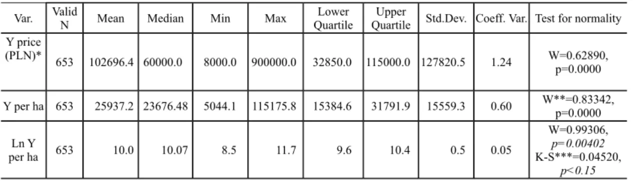
The linear multilevel analysis is a supplement to standard linear regression analysis. Hence the continuous output variable ought to have a normal distribu- tion. Some tests show that this assumption is fulfilled at p=0.05, while others indicate that it is not (Table 1). The distribution of the dependent variable may therefore deviate slightly from normal, but this should not have a significant ef- fect on the results. Descriptive statistics for the dependent variable and the inde- pendent ones are given in Tables 1 and 2, respectively, while the comparison of the estimated models is presented in Table 3.
Table 1. Descriptive statistics of the dependent variable Var. Valid
N Mean Median Min Max Lower
Quartile Upper
Quartile Std.Dev. Coeff. Var. Test for normality Y price
(PLN)* 653 102696.4 60000.0 8000.0 900000.0 32850.0 115000.0 127820.5 1.24 W=0.62890, p=0.0000
Y per ha 653 25937.2 23676.48 5044.1 115175.8 15384.6 31791.9 15559.3 0.60 W**=0.83342, p=0.0000 Ln Y
per ha 653 10.0 10.07 8.5 11.7 9.6 10.4 0.5 0.05
W=0.99306, p=0.00402 K-S***=0.04520,
p<0.15 Notes: *average exchange rate €1 = 4.17 PLN; **Shapiro–Wilk test; ***Kolmogorov–Smirnof test.
Table 2. Descriptive statistics of the explanatory variables
Average Min Max Standard deviation
ara&LFA paym 0.36 0.00 1.00 0.48
area paym. only 0.35 0.00 1.00 0.48
area&env paym. 0.05 0.00 1.00 0.23
area&LFA&env paym. 0.09 0.00 1.00 0.28
areas of agroturistic type 0.10 0.00 1.00 0.30
areas of city integrated type 0.25 0.00 1.00 0.43
areas of competitive agriculture 0.09 0.00 1.00 0.28
areas of peripheral type 0.56 0.00 1.00 0.50
asphalt road 0.37 0.00 1.00 0.48
building possibilities 0.36 0.00 1.00 0.48
dist. to building (m) 218.57 0.00 3 860.00 459.53
dist. to city (km) 7.23 0.20 26.70 4.03
land productivity coeff. 46.05 0.00 94.00 22.42
peripheral area 0.57 0.00 1.00 0.50
shape coeff. 2.60 1.00 5.00 1.42
surface area (ha) 3.84 1.00 25.96 3.79
without payment 0.15 0.00 1.00 0.35
year2010 0.17 0.00 1.00 0.37
year2011 0.24 0.00 1.00 0.43
year2012 0.28 0.00 1.00 0.45
year2013 0.31 0.00 1.00 0.46
Source: Own elaboration based on data from registers of features and values of properties maintained by county (poviat) authorities, land register information from the National Geoportal, and agricultural soil maps from the Provincial Geodetic and Cartographic Repository.
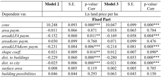
Table 3. Fixed and random parts of the models Model 2 S.E. p-value/
Corr Model 3 S.E. p-value/
Corr
Dependent var. Ln land price per ha
Fixed Part
cons 10.248 0.093 0.000*** 10.047 0.099 0.000***
area paym. –0.011 0.066 0.871 0.018 0.065 0.784
area&LFA paym. –0.152 0.060 0.011** –0.169 0.058 0.004***
area&env paym. 0.030 0.099 0.760 0.071 0.099 0.476
area&LFA&env paym. –0.231 0.084 0.006*** –0.214 0.081 0.008***
shape coeff. 0.021 0.009 0.016** 0.012 0.007 0.090*
dist. to buildings –0.229 0.060 0.000*** –0.280 0.053 0.000***
dist. to city –0.025 0.006 0.000*** –0.021 0.006 0.000***
surface area 0.008 0.005 0.119 0.002 0.005 0.705
building possibilities 0.046 0.044 0.293 0.063 0.043 0.150
5. RESULTS AND DISCUSSION
The market for agricultural land in the Wielkopolska region exhibits very high degree of variations: the average price of a purchased property was 103,000 Polish Zloty (PLN), median 60,000 PLN with a standard deviation of 128,000 PLN, and a coefficient of variation of 1.24. The price per hectare is less variable:
its mean is 26,000 PLN (median 24,000 PLN) with standard deviation 16,000 PLN (coefficient of variation is 0.6). Neither of these two variables has a normal distribution (Shapiro-Wilk tests lead to rejection of the hypothesis of normality
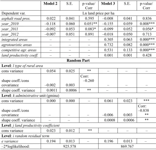
Table 3. cont.
Model 2 S.E. p-value/
Corr Model 3 S.E. p-value/
Corr
Dependent var. Ln land price per ha
asphalt road prox. 0.022 0.041 0.595 –0.008 0.041 0.836
year_2010 –0.118 0.060 0.051** –0.155 0.059 0.008***
year_2011 –0.092 0.053 0.083* –0.099 0.052 0.056*
year_2012 –0.007 0.051 0.891 –0.018 0.050 0.713
integrated areas – – – 0.305 0.063 0.000***
agrotouristic areas – – – 0.732 0.082 0.000***
competitive agr. areas – – – 0.531 0.133 0.000***
land productivity coeff. – – – 0.001 0.001 0.428
Random Part Level: l type of rural area
cons variance 0.054 0.025 ** – – –
shape coeff./cons
covariance –0.002 0.003
Corr:
–0.260
– – –
shape coeff. variance 0.0011 0.0006 ** – – –
Level: k administrative unit (gmina)
cons variance 0.000 0.000 – 0.061 0.023 ***
shape coeff./cons
covariance – – – –0.006 0.003
Corr:
–0.838
**
shape coeff. variance – – – 0.0008 0.0006 **
Level: j land productivity coefficient
cons variance 0.023 0.012 ** – – –
Level: i random residual term
e variance 0.194 0.013 – 0.196 0.013 –
–2*loglikelihood: 925.578 869.767
Note: ***,**,* significance levels at 1%, 5%, 10%, respectively.
Source: Own computations using MLwiN 2.36 (Centre for Multilevel Modelling, University of Bristol).
at p<0.0001); they both exhibit right-handed asymmetry (strongly, in the case of prices per property). In the log-linear version of the model, however, the distribu- tion of ln Y per ha is close to normal, as mentioned above (Table 1). It was also found that the set of explanatory variables at the transaction level, excluding the location-specific factors, explain the variation in prices per ha to a relatively small degree (the coefficient pseudo-R2 was below 0.3). This can be partially ascribed to speculation on the land market and the significant demand disequilibrium, but it is the three location-specific factors in this case that have a key impact: agri- cultural complex, administrative unit (gmina) and rural area type. The solution to this problem is therefore the use of hierarchical modelling.
We undertook an attempt to model land prices per ha, to make it easier to inter- pret the marginal effects of particular variables. In the first step, we computed the set of equations and variance/covariance matrices shown in Equation 2. Statisti- cally significant variables are asterisked, and standard errors are in parentheses.
There is also detailed description of fixed and random parts in Table 3.
0 5
0 0 0 0 0
5 5
2 2
0 0 0
2 2
0 0 0
10.248(0.093) 0.021(0.009)
0.054 0.025
0.002 0.003 0.0011 0.0006
~ (0, ) 0.000(0
~ N(0,
.000)
~ (0, ) 0.023(0.012)
~
):
jl l kl jkl
l l
kl v v
jkl u u
ij l
f
kl
f l
f v u
f
v N
u N
e
f f
β β
β
σ σ σ σ
Ω Ω
2 2
(0, e) 0.194(0.013)e
N σ σ
–2*loglikelihood=925.578 (653 of 653 cases in use, MLwiN, version 2.36.)
(2)
where: SE in parentheses; i – ordinal; l – type of rural area**; k – administrative unit (gmina); j – agricultural complex**; ***p < 0.001,** p < 0.05, * p < 0.1
Statistical significance was found for the introduction of two levels of analy- sis, which was checked by comparing the statistic–2*loglikelihood for different
5
0 0.011(0.066) . 0.152(0.060) & .
0.030(0.099) & . 0.231(0.084) & & .
. 0.229(0.060) .
per ijkl jkl ijkl ijkl
ijkl ijkl
ijkl
lny ha area paym area LFA paym
area env paym area LFA env paym
shape coeff dist to build
β β
2010 2011
0.025 0.006 . 0.008(0.005)
0.046 0.044 0.022(0.041) .
0.118 0.060 0.092(0.053)
0.007
ijkl
ijkl ijkl
ijkl ijkl
ijkl ijkl
ings
dist to city surface
building possibilities asphalt road prox
year year
(0.052)year2012ijkleijkl
model versions. The location-specific factor “type of rural area” is significant at p < 0.05, and “agricultural complex” (j) is significant at p < 0.1. In this case the administrative unit (gmina) level proved insignificant. Moreover, the random regression coefficient for the shape coefficient significantly improves the fit of the model. The variable f5l in the nested function is also statistically significant.
We recall that the variable shape coeff. shall be important to explain the value of farmland since it comprises the fragmentation of land. In higher fragmented plots (lower shape coeff.), the agricultural use is more limited. We therefore computed the intra-class correlation coefficient (ICC) based on the variance of the free terms and the remaining residual variance for the significant levels of analysis, obtain- ing the value 0.284. This means as much as 30% of the model’s unobserved het- erogeneity can be ascribed to the grouping variables: about 20% to the rural area type and about 10% to the “agricultural complex” (coefficient of land productiv- ity). This is a relatively high value as in the single-level model the explanatory variables explained approximately 30% of the variation in prices per ha. Confir- mation was thus obtained for the hypothesis that the location-specific factors are key drivers for land prices, with rural area type being the most significant factor.
Next, using Wald’s test, we determined which of the explanatory variables are statistically significant. The figures in brackets are the standard errors for the re- gression coefficients. By computing the EXP function for particular coefficients, their marginal effect can be evaluated precisely. The analysis was performed with a division according to parcel-level attributes and the effect of agricultural policy (payments for public goods). Statistically significant attributes have the follow- ing marginal effects (EXP function for particular coefficients minus 1): improve- ment in the shape coefficient by one unit increases the price per ha by 2.1%; an increase in distance to buildings by 1 km reduces the price per ha by 20.5%; an increase in distance to the city by 1 km reduces the price per ha by 2.5%; transac- tions concluded in 2010 had a price per ha lower by 10.9% than in 2013; trans- actions concluded in 2011 had a price per ha lower by 9.4% than in 2013; and transactions concluded in 2012 had a price per ha lower by 1.8% than in 2013.
Statistically significant policy variables were found for additional LFA pay- ments and sustainable support combining single area payment and LFA with agri-environmental payments (area&LFA and area&LFA&env), but their mar- ginal effects are negative: receipt of additional LFA payments reduces the price per hectare by 15.5%, while ES reduces it by 19.3%. This shows that the limita- tions on farming use (both natural and enforced by the CAP) associated with the receipt of these payments might have a negative effect on land rent and restrict possibilities of earning.
The direction of influence is logical. The results imply that location, distance from the city and infrastructure are key factors for agricultural land prices and
exert a much stronger marginal effect than the hedonic features contained in the shape coefficient. It is in the line with other researches which have identified land value as a negative exponential function of the distances to large cities and the nearest city with at least 10,000 residents (Tsoodle et al. 2007). Similar con- clusions have been formulated based on gravity models which measure urban influence by dividing county population by the squared distance of a county from business districts, as well as including both population and real income in urban areas (Guiling et al. 2009).
The results are somewhat surprising and contradict popular opinions about the effect of agricultural policy on land prices in Poland. Firstly, the effect of separate single area payments (area paym.) is statistically insignificant which is in line with some findings for Western Europe. Under the BPS, farmers are required to maintain the area of land on which they claim their single payment in good agricultural and environmental condition. This requirement is termed as ‘cross-compliance’. The land area to be maintained is equal to the average number of hectares declared by the farmer in the reference period of 2000–2002 for which they had received their single-payment entitlements. The cited authors argue that the ‘cross-compliance’
obligations are sufficient to prevent farms from changing their land market deci- sions due to the increase of overall wealth (land collateral) and easier provision of loans from banks (Rude 2000), although farmers’ risk aversion decreases (Hen- nessy 1998; Koundouri et al. 2009). As a result the decoupled payments support on-farm investment and off-farm labour supply (Guyomard et al. 2004) rather than farmland purchases. Thus, one may anticipate a negligible impact of decoupling reform both on farmers’ demand for land and on-land supply, since farmers who have acquired land in the reference period would be forced to maintain that level of land to satisfy the cross-compliance requirements (O’Neill – Hanrahan 2012), while they have few opportunities to gain additional entitlements. For that reason, a petrifaction of farmland structure under the BPS will occur, and land prices will not be subjected to a long-term upward tendency. Under the SAPS the land market situation is quite different for the new member countries in the EU-12. Farmers do not need any historical entitlements for payments because mere possession of land entitles them to receive subsidies. As a result, a growing demand for farmland occurs, especially in agricultural regions where the phenomenon of ‘land hunger’
arises. However, the basic area payments have been already discounted on land prices, considering that the subsidy for each hectare had been known in advance before the beginning of each CAP operating period.
The farm real estate accounts for more than 80% of the total value of the United States farm assets, being a principal source of collateral for farm loans (Nickerson et al. 2012). If this were the case, feedback demand for land would oc- cur, boosting its prices (MacDonald et al. 2013). Breustedt – Habermann (2011)
found evidence that a farmland bubble would occur if the collateral helped farm- ers obtain more or cheaper financing, amplifying an initial increase in land prices, with a land-related increase in wealth leading to higher borrowing to buy land, which further increases land prices and collateral (see also Rajan – Ramcharan 2012). These factors have caused dramatic increases in farmland values in the US, where from 2004 to 2012 nominal cropland values doubled (USDA-NASS 2012). Lowenberg-DeBoer – Boehlje (1986) showed that capital gains from farm- land appreciation increase a farmer’s collateral. But it is not the case in Poland because banks are not willing to accept land as collateral. However, the situation when farmers pass on a considerable share of payments to landowners via farm- land rental rates or informal channels is very typical in Poland, and then the pay- ments do not capitalise as cited by Karlsson – Nilsson (2013). Last two factors might be the reasons for the insignificant coefficient of the single area payment in the model. We also recall that the expectations to increase in land prices are already discounted, and in most places at present, single payment support is not a differentiating factor for land value.
Interesting conclusion is that the other payments (area&LFA and area&LFA&env) might not compensate for the opportunity costs related to al- ternative ways of land use as it is expected in CAP assumptions. Although the finding is contradictory to the studies cited above, some authors came to the same conclusion. According to Nilsson – Johansson (2013), agricultural and environ- mental payments in Sweden have also a negative influence on land prices. They argue that municipalities receiving agri-environmental support have very sensi- tive environments which are difficult for cultivation. A similar conclusion was reached in a previous study by Rutherford et al. (1990).
However, these effects have to be interpreted with a caution. An additional discussion is needed on the potential misleading effect of an endogenous allo- cation of LFA and environmental payments. Are the land prices lower due to agri-environmental support, as it was stated by the cited authors, or is it because of the difficulty to cultivate? There is a logical shortcut in this reasoning. In our opinion, the estimated negative effects can be casual, but only to some extent.
The allocation of environmental payments is based on some characteristics cor- related with land prices. Let us discuss it with the example of the most popular environmental schemes in Wielkopolska (Greater Poland) region: “Package 1.
Sustainable farming” and “Package 2. Protection of soil and water”. The first one had very demanding (and costly) requirements which theoretically could affect the land price, i.e.: the obligation to maintain all the permanent grassland and landscape elements not used for agricultural purposes unchanged, the ban on the sewage sludge use, the ban on the resuming agri-technical treatments before 15 February and the obligation to have a 5-year agri-environmental plan. The sec-
ond scheme similarly implemented the ban on agri-technical treatments before 1 March and the ban on using a mixture of plants consisting of only species of cere- als (Ministry of Agriculture and Rural development 2016). We have to consider questions like; why farmers decided to apply for these payments and whether removing the payments would increase the price of the land? In Wielkopolska, there are not many natural obstacles to farming, the fertile plains dominate. How- ever, one can find valuable ecosystems along the bends of rivers and close to wooded areas being wildlife refuges. They are usually covered by the Nature 2000 network, and it is very difficult to obtain a building permission for any new facilities there. If some agricultural plots are located in such areas, the easiest way to retrieve a land rent is applying for environmental payments. Then, the requirements of CAP programmes sustain the status quo and a land is perceived by investors as less valuable. So, without these payments, it would be more likely that some economic activities occur nearby, thus busting the land prices. Hence, we believe that in case of Poland the payments for public goods are probably too low and fail to perform their role of compensating for the opportunity costs of pro-environmental land use.
Considering that the model described in Equation 2 indicates rural area type as the key factor explaining variation in land prices, we computed a second model (Equation 3), including the four types of area in the set of explanatory variables.
This was done to determine which types of the rural area most strongly drive land prices, and in what direction. As has already been mentioned, each type is linked to different use values and amenities of agricultural land. In the case of agro-touristic areas, these are chiefly touristic and recreational amenities, for city-integrated areas they are urban amenities, and for areas of competitive agri- culture they chiefly use values (the effect of peripheral areas is contained in the free term). The model in Equation 3 shows their final effect on land prices:
0
12 0.053
0.018(0.065) . 0.169(0.058) & . 0.071(0.099) & . 0.214(0.081) & & .
. 0.280( ) .
0.02
per ik k ik ik
ik ik
ik ik
ny ha area paym area LFA paym
area env paym area LFA env paym
shapecoeff dist tobuildings
β β
1(0.006) . 0.002(0.005)
0.063(0.043) 0.008(0.041) .
0.305(0.063) 0.732(0.082) 0.
ik ik
ik ik
ik ik
dist to city surface
building possibilitiesYES asphalt road prox city integrated area agrotouristic area
531(0.133) 0.115(0.059) _ 2010 0.099(0.052) _ 2011 0.018(0.050) _ 2012 0.001(0.001) .
ik ik
ik ik
ik ik
competitive area year
year year
productivity coeff e
(3)