Paper No. §§§
Abstract. Empirical liquefaction potential assessment is generally based on the results of CPT, SPT or shear wave velocity (VS) measurement. In more complex or high-risk projects CPT and VS measurement are often performed at the same location commonly in the form of seismic CPT. However, combined use of both in-situ indices in one single empirical method has been limited. After the compilation of a case history database, the authors have developed a combined probabilistic method where the results of CPT and VS measurement can be used in parallel.
The goal of this paper was to evaluate the prediction capability of the developed equation on an independent dataset of the 2010-2011 Canterbury Earthquake Sequence and to compare it with commonly used empirical procedures. It was found that the error index defined to quantify the false predictions is the largest for the recommended method but regarding the number of false predictions, it outperforms the other methods used for comparison.
Keywords: Liquefaction; CPT; Shear Wave Velocity; Prediction
1 INTRODUCTION
Soil liquefaction is one of the most devastating secondary effects of earthquakes and can cause considerable damage in the built infrastructure. Several approaches exist to quantify this hazard, from which the in-situ test based empirical methods are the most commonly used in practice. Traditional means of these tests are the Standard Penetration Test (SPT), Cone Penetration Test (CPT) and shear wave velocity (VS) measurement. In more complex or high-risk projects, CPT and VS measurement are often performed at the same location, commonly in the form of Seismic Cone Penetration Test (sCPT).
However, even if the results of the two tests are available for the same spot, empirical liquefaction potential evaluation can be performed using either of them, but combined use of the data in one single method has been limited. In order to surmount this issue, an attempt has been made to develop an empirical method, which exploits both the results of CPT and VS measurement. The effort is based on the assumption that these soil properties complement each other since they characterize the behaviour of granular systems at different levels of strain.
2 LIQUEFACTION POTENTIAL ASSESSMENT BASED ON CONE PENETRATION TESTING AND SHEAR WAVE VELOCITY MEASUREMENT
Since the introduction of cyclic shear stress approach (Seed and Idriss 1971), several empirical methods have been published by different authors that can give a relatively reliable quantification of liquefaction hazard by determining factor of safety or probability of liquefaction occurrence. In current engineering practice, the most commonly used CPT-based methods are the procedures proposed by Robertson and Wride (1998), Moss et al. (2006), Idriss and Boulanger (2008) and Boulanger and Idriss (2014). As the use of CPT for ground profile characterization is very popular, its application for liquefaction potential evaluation is also prevalent.
Performance of Liquefaction Assessment Method Based on Combined Use of Cone Penetration Testing and Shear Wave Velocity Measurement
BÁN Zoltán1, MAHLER András2, GYŐRI Erzsébet3
1 M.Sc., Ph.D. stud., Budapest Uni. of Technology, Műegyetem rkp. 3, Budapest, 1111, ban.zoltan@epito.bme.hu
2 Ph.D., Assoc. Prof., Budapest Uni. of Technology, Műegyetem rkp. 3, Budapest, 1111, mahler@mail.bme.hu
3 Ph.D., Sr. Res. Fel., MTA CSFK GGI Kövesligethy Radó Seism. Observatory, Budapest, gyori@seismology.hu
Compared to CPT- and SPT- based methods, the procedures based on VS tests are less widely used in practice. For very long time, the method of Andrus and Stokoe (2000) was used almost exclusively.
Very recently, the work of Kayen et al. (2013) made a huge step in the advancement of VS-based methods. Besides the advanced statistical framework adopted by the authors, the most remarkable accomplishment was the compilation of a global catalogue of 422 case histories.
3 DEVELOPMENT OF A COMBINED CONE PENETRATION TEST- AND SHEAR WAVE VELOCITY-BASED METHOD
3.1 Field case history dataset
The first and most time-consuming step of the development was the collection of a liquefaction/non- liquefaction field case history catalogue. Through careful review of existing CPT and VS databases, 98 cases were found where both measurements are available. As locations where liquefaction occurred are more enticing for post-earthquake field investigators than sites where no apparent liquefaction occurred, the assembled dataset over represents liquefied sites (68 sites), relative to non-liquefied sites (30 sites).
The core of the database was assembled from the CPT case history catalogue of Moss et al. (2006) and VS dataset of Kayen et al. (2013), from which 73 and 53 locations could be used, respectively. Additional case histories were gathered from the publications of various authors. For complete list of the used literature, see Bán et al. (2016). The final database consists case histories from 12 earthquakes (1975 Haicheng, 1976 Tangshan, 1979 Imperial Valley, 1981 Westmoreland, 1983 Borah Peak, 1987 Elmore Ranch, 1987 Superstition Hills, 1989 Loma Prieta, 1999 Chi-Chi, 1999 Kocaeli, 2008 Achaia-Elia, 2011 Great Tohoku).
3.2 Input parameters and their normalization
According to the framework of simplified empirical procedures, the seismic demand induced by an earthquake can be represented by the cyclic stress ratio (CSR). This parameter is generally corrected to 7.5 magnitude and 1 atm effective vertical stress to take into account duration – or number of equivalent cycles – of different earthquakes and the dependency of cyclic liquefaction on effective overburden stress. For these corrections, the method and equations of Idriss and Boulanger (2008) was followed.
Effective overburden stress can also profoundly influence CPT measurements. This effect is typically accounted for by normalizing the tip resistance measured at a given depth to a reference effective stress of 100 kPa. Similarly to CSR, the procedure recommended by Idriss and Boulanger (2008) was followed to take into account this effect. The role of fines on liquefaction susceptibility is a somewhat contentious topic. Nevertheless, it is agreed that if the fines content (FC) exceeds approximately 35-40% the coarser grains will “float” in the matrix of fine-size particles and the cyclic behaviour of the soil will be governed by the fines. For the development of the equation, equivalent clean sand values of the tip resistance were determined using the updated equation of Boulanger and Idriss (2014). As well as CPT tip resistance, VS is also routinely normalized to an equivalent value measured at 100 kPa effective overburden stress (Robertson et al. 1992). VS measurement is not capable of detecting small differences in fines content, i.e. VS is relatively insensitive to FC. Compared to uncertainties arising from other parts of the methodology this correction would be fairly negligible; thus, fines content correction of the shear wave velocity was neglected.
After performing all of the above discussed normalization and corrections, three explanatory variables remained to participate in the logistic regression: the equivalent clean sand value of normalized overburden corrected cone tip resistance (qc1Ncs), the overburden corrected shear wave velocity (VS1), and the magnitude and the effective stress corrected cyclic stress ratio (CSRM=7.5,σ’v=1atm).
3.3 Logistic regression
Logistic regression is often used to explore the relationship between a binary response and a set of explanatory variables. The occurrence or absence of liquefaction can be considered as binary outcome and the previously summarized three parameters are the explanatory variables. The key components of the regression are the formulation of a limit state model that has a value of zero at the limit state and is negative and positive for liquefaction and non-liquefaction cases, respectively, and a likelihood function that is proportional to the conditional probability of observing a particular event assuming a given a set of parameters. The approach of Cetin et al. (2002) was adopted to form the limit state function.
Assuming the statistical independence of the observations compiled from different sites, the likelihood function can be written as the product of the probabilities of the observations. As it was noted in section 3.1, the dataset contains significantly more liquefaction cases than non-liquefaction cases; this bias is undesirable in logistic regression and can adversely affect the result. A way to address this issue is to weight each class of cases according to the proportion of the other’s class population in the total database (Cetin et al. 2002). After taking the natural logarithm of the likelihood function that is more convenient to work with, the unknown parameters were determined using maximum likelihood estimation.
3.4 Probability of liquefaction
The logistic regression using the likelihood function yielded the following result:
𝑃𝐿= 𝜃 [0.080∙𝑉𝑠1+0.177∙𝑞𝑐1𝑁𝑐𝑠−8.40∙𝑙𝑛(𝐶𝑆𝑅𝑀=7.5,𝜎′𝑣=1𝑎𝑡𝑚)−46.04
3.46 ] (1)
where Θ is the standard normal cumulative probability function. The denominator, that is the standard deviation of the error term, is of particular interest since it describes the efficiency of the liquefaction relationship. The regressed value is somewhat higher than that of other commonly used methods, but the method is still promising, since this method has seen little refinement so far. The cyclic resistance ratio for a given probability of liquefaction can be expressed by rearranging Equation 1:
𝐶𝑆𝑅𝑀=7.5,𝜎′𝑣=1𝑎𝑡𝑚= 𝑒𝑥𝑝 [0.080∙𝑉𝑠1+0.177∙𝑞𝑐1𝑁𝑐𝑠−46.04+3.46∙𝜃−1(𝑃𝐿)
8.40 ] (2)
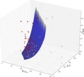
This can be used in deterministic analysis by selecting a probability contour (typically PL= 15%) to separate liquefaction and non-liquefaction states. Figure 1 shows the probability surface corresponding to PL = 50%.
More detailed description of the complied dataset and the development the above equations can be found in Bán et al. (2016).
4 2010-2011 CANTERBURY EARTHQUAKE SEQUENCE
The 2010–2011 Canterbury earthquake sequence began with the 4 September 2010 Mw 7.1 Darfield earthquake and included up to ten events that induced liquefaction. However, most notably, widespread liquefaction was induced by the Mw 7.1, 4 September 2010 Darfield and the Mw 6.2, 22 February 2011 Christchurch earthquakes. The ground motions from these events were recorded across Christchurch and its environs by a dense network of strong motion stations. Also, due to the severity and spatial extent of liquefaction resulting from the 2010 Darfield earthquake, an extensive subsurface characterization program took place with over 10,000 CPT soundings (Green et al. 2014).
Figure 1. Cyclic resistance ratio surface corresponding to 50% of liquefaction probability (solid squares – liquefaction cases, hollow circles – non-liquefaction cases).
The combination of well-documented liquefaction response during multiple events, densely recorded ground motions for the events, and detailed subsurface characterization provided an unprecedented opportunity to add numerous quality case histories to the liquefaction database. The paper of Green et al. (2014) presented 50 high-quality CPT test liquefaction case histories which consisted of 25 sites analysed for both the Darfield and Christchurch earthquakes. Besides, the compilation of quality liquefaction data, their goal was to compare and evaluate commonly used, deterministic, CPT-based liquefaction evaluation procedures. An error index was used to quantify the overall performance of the procedures in relation to liquefaction observations. It was concluded that among them, the procedure proposed by Idriss and Boulanger (2008) results in the lowest error index for the case histories analysed, thus indicating better predictions of the observed liquefaction response.
In a subsequent research of the same authors (Wood et al. 2017), they examined 46 of the 50 case histories using shear-wave velocity profiles derived from surface wave methods. The VS profiles have been used to evaluate the two most commonly used Vs-based simplified liquefaction evaluation procedures (Andrus and Stokoe and Kayen et al.). It was found that the Kayen et al. procedure outperforms the Andrus and Stokoe procedure but has slightly worse performance than that of the CPT- based Idriss and Boulanger method.
The compiled case histories of the Canterbury Earthquake Sequence and the fact that they were explored by both CPT and Vs measurement provide an excellent opportunity for the verification of the developed combined method and comparison with the most commonly used and best performing CPT- and VS- based methods (i.e. with the procedures of Idriss and Boulanger and Kayen et al.).
5 EVALUATION OF PROCEDURES
The papers of Green et al. (2014) and Wood et al. (2017) define an error index to quantitatively assess which liquefaction evaluation procedure yields the “most accurate” predictions for the data analysed.
The two error indices used by the two papers are slightly different due to the nature of the CPT- and Vs- based procedures (i.e. the catalogue of the VS-based method of Kayen et al. didn’t have wide enough range to properly account for the Kσ effect, which is in the other hand incorporated into the CPT-based method of Idriss and Boulanger). The proposed error indices equal zero if all the predictions correctly
match the field observations but increase in value as the number and “magnitude” of the mispredictions increases.
For present study a similar concept was adopted to compare the different methods’ prediction capability.
The aforementioned indices can be illustrated as the vertical distance between the CRRM7.5 / CRRM7.5,σ’v=1atm curve and the plotted mispredicted point. To allow direct comparison of the methods and to adopt a slightly more straightforward approach, not the vertical distance from the CRR curve were used for quantification, but mispredictions were quantified in terms of factor of safety. On an individual case basis, the error index (EI) equals zero for a correct prediction of a Liquefaction or No Liquefaction case and equals the absolute value of 1 minus FS for mispredicted cases. Similarly to the paper of Wood et al. (2017), to acknowledge the varying significance of the consequences of mispredicting cases, weighting factors are included in the error index: 1.0 for mispredicted liquefaction cases, and 0.5 for mispredicted no Liquefaction cases (Eq. 3).
𝐸𝐼 = 0 for correct prediction (3)
𝐸𝐼 = 𝐹𝑆 − 1 for mispredicted liquefaction case
𝐸𝐼 = 0.5 ∙ (1 − 𝐹𝑆) for mispredicted no liquefaction case
The computed error index values for the 46 case histories are summarized in Table 1. Please note that the values of error indices are different from those presented in Green et al. (2014) and Wood et al.
(2017) due to the different error index definition. Green et al. (2014) and Wood et al. (2017) categorized the cases based on their severity as “no liquefaction”, “minor liquefaction”, “moderate liquefaction” and
“severe liquefaction” cases. For this study, the latter 3 cases were considered as simply liquefaction cases and the first category was obviously the no liquefaction case.
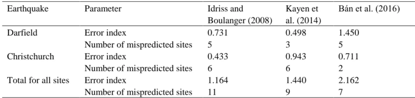
Table 1. Error index and number of mispredicted sites for the three evaluated liquefaction evaluation procedures
Earthquake Parameter Idriss and
Boulanger (2008)
Kayen et al. (2014)
Bán et al. (2016)
Darfield Error index 0.731 0.498 1.450
Number of mispredicted sites 5 3 5
Christchurch Error index 0.433 0.943 0.711
Number of mispredicted sites 6 6 2
Total for all sites Error index 1.164 1.440 2.162
Number of mispredicted sites 11 9 7
As the table shows the equation of the authors has the highest error index term, so it has the worst prediction capability among the three examined methods. As it is concluded by Wood et al. (2017) and also confirmed by present comparison, the total error values obtained using Kayen et al. (2013) Vs- based procedure is higher than that of the Idriss and Boulanger (2008) CPT-based procedure indicating slightly better performance of the latter method. However, if one considers not the error index but the number of mispredicted sites, in that case the equation recommended by the authors outperforms the other two procedures. The higher error index of the authors’ equation is mostly resulted by mispredicted no liquefaction sites for which both the CPT- and VS-based method predicted liquefaction with factors of safety around 0.6-0.8. As both measurements predicted false response, the recommended formula based on both CPT and VS also predicted false response but due to the combination of them, its factor of safety is much lower, around 0.3-0.4. On the other hand, during the Christchurch earthquake the CPT- and VS-based procedures predicted no liquefaction for some liquefied site (FS around 1.0-1.1), for which the recommended combined formula predicted correct response. Due to these factors the recommended combined equation predicted less false responses but where false prediction occurred, the magnitude of error was considerably higher than that of Idriss and Boulanger CPT- or Kayen et al. VS-based method.
6 CONCLUSIONS
More increasingly CPT and VS measurement are often performed on the same location however the possibility to characterize liquefaction potential with both indices in one single empirical method was limited so far. The main goal of the presented research was to develop such a method within the framework of simplified empirical procedures that can reduce uncertainty of empirical methods by combining the two in-situ indices; a small strain property measurement with a large strain measurement.
After compiling a case history dataset where both measurements are available and implementing the necessary corrections on the gathered case histories with respect to fines content, overburden pressure and magnitude, a logistic regression was performed to obtain the probability contours of liquefaction occurrence. The proposed formula is an initial attempt to exploit the advantages offered by the measurements of two soil parameters instead of one.
The goal of this paper was to evaluate the prediction capability of the developed equation on an independent dataset of the 2010-2011 Canterbury Earthquake Sequence and to compare it with commonly used empirical procedures. This was performed by means of an error index similar to those defined by Green et al. (2014) and Wood et al. (2017). It was shown that compared to the state-of- practice CPT-based empirical method of Idriss and Bulanger and VS-based method of Kayen et al., the recommended combined equation of the authors has much higher error index, so it has the worst prediction capability among the three examined methods, but if the number of mispredicted sites is considered, it outperforms the other two procedures. The obtained results are promising, since the author’s method has seen very little refinement so far, especially compared to the other two methods.
REFERENCES
Andrus, R.D. and Stokoe, K.H., II. (2000). Liquefaction resistance of soils from shear-wave velocity. Journal of Geotechnical and Geoenvironmental Engineering 126(11): 1015–1025.
Bán Z., Mahler A., Katona T.J. and Győri E. (2016).Liquefaction assessment based on combined use of CPT and shear wave velocity measurement, In: Lehane B.M., Acosta_Martínes A.E. and Kelly. R. (eds), Proceedings of 5th International Conference on Geotechnical and Geophysical Site Characterization, Gold Coast, 5-9 September 2016. pp. 597-602
Boulanger, R.W. and Idriss, I.M. (2014). CPT and SPT based Liquefaction Triggering Procedures. Report No.
UCD/CGM-14/01, University of California, Davis.
Cetin, K.O., Der Kiureghian, A. and Seed, R.B. (2002). Probabilistic models for the initiation of seismic soil liquefaction. Structural Safety 24(1): 67–82.
Green, R. A., et al. (2014). Select liquefaction case histories from the 2010–2011 Canterbury earthquake sequence.
Earthquake Spectra, 30(1), 131–153.
Idriss, I.M. and Boulanger, R.W. (2008). Soil Liquefaction during Earthquakes. Monograph MNO-12, Earthquake Engineering Research Institute, Oakland.
Kayen, R., Moss, R.E.S., Thompson, E.M., Seed, R.B., Cetin, K.O., Der Kiureghian, A., Tanaka, Y. and Tokimatsu, K. (2013). Shear-Wave Velocity–Based Probabilistic and Deterministic Assessment of Seismic Soil Liquefaction Potential. Journal of Geotechnical and Geoenvironmental Engineering 139(3): 407-419.
Moss, R.E.S., Seed, R.B., Kayen, R.E., Stewart, J.P., Der Kiureghian A. and Cetin, K.O. (2006). CPT-based probabilistic and deterministic assessment of in situ seismic soil liquefaction potential. Journal of Geotechnical and Geoenvironmental Engineering 132(8): 1032–1051.
Robertson, P.K., Woeller, D.J., and Finn, W.D.L. (1992). Seismic cone penetration test for evaluating liquefaction potential under cyclic loading. Canadian Geotechnical Journal 29(4): 686–695.
Robertson, P.K. and Wride, C.E. (1998). Evaluating cyclic liquefaction potential using the cone penetration test.
Canadian Geotechnical Journal 35(3): 442-459.
Seed, H.B. & Idriss, I.M. (1971). Simplified procedure for evaluating soil liquefaction potential. Journal of the Soil Mechanics and Foundations Division 97(SM9): 1249-1273
Wood, C.M., Brady, R.C., Green, R.A, Wotherspoon R.M., Bradley, B.A and Cubrinovski, M. (2017). Vs-Based Evaluation of Select Liquefaction Case Histories from the 2010-2011 Canterbury Earthquake Sequence.
Journal of Geotechnical and Geoenvironmental Engineering 143(9): 04017066.