Single Determinant Basis Set for the Non-Relativistic Electronic Schrödinger Equation Using the Coupling Strength Parameter Generalized Brillouin Theorem
Sandor Kristyan
Research Centre for Natural Sciences, Hungarian Academy of Sciences, Institute of Materials and Environmental Chemistry
Magyar tudósok körútja 2, Budapest H-1117, Hungary, Corresponding author: kristyan.sandor@ttk.mta.hu
Abstract. The Brillouin theorem has been generalized for the coupling strength parameter (a) extended non-relativistic electronic Hamiltonian (HHne+aHee). The mathematical case a=0 generates an orto-normalized set of single Slater determinants which can be used as basis set for configuration interactions (CI) calculations for the physical case a=1, removing the known restriction by the original Brillouin theorem and opening a new way to practice.
Keywords. electron-electron repulsion energy participation in ground and excited states, coupling strength parameter, totally non-interacting reference system, generalization of Brillouin theorem, single determinant basis set, configuration interactions
INTRODUCTION: Coupling strength parameter as input
The non-relativistic, spinless, fixed nuclear coordinate electronic Schrödinger equation for a molecular systems of M atoms and N electrons with nuclear configuration {RA, ZA}A=1,…,M in free space is
H(a) yk (HHne+ aHee) yk(x1,…,xN) = enrgelectr,k yk(x1,…,xN) (1) where yk and enrgelectr,k are the kth excited state (k=0,1,2,...) anti-symmetric wave function (with respect to all spin- orbit electronic coordinates xi ≡ (ri,si)) and electronic energy, respectively, as well as the electronic Hamiltonian operator contains the sum of kinetic energy, nuclear–electron attraction and electron–electron repulsion operators, the latter is extended with coupling strength parameter (a). Only a=1 makes physical sense (!), while the case a=0 mathematically provides a good starting point to solve the case a=1. Most popular approximations [1, 2] are the expensive but (chemical) accurate CI method for ground and excited states, the less accurate but faster and less memory taxing Hartree–Fock self consistent field (HF-SCF) method for ground state with or without correlation corrections, and the density functional theory (DFT, using HF-SCF framework) [3]. The CI works for any nuclear geometry, while the HF-SCF is only for the vicinity of stationary points using a single Slater determinant. The “a”
connects an unphysical system (H(a=0)) to the system treated at the mean-field HF level (H(a=1)) and above and its effect on ground and excited states. For example, a bit below unity “a” is capable [4] to correct the HF-SCF energy remarkably.
The (yk(a),enrgelectr,k(a)) is the k-th eigenvalue pair of H(a), and we distinguish notations for a=0 as (Yk,eelectr,k) and for a=1 as (k,Eelectr,k). The S0 (generally s0(a)) is a single determinant approximation for 0 (generally for y0(a)) via HF-SCF/basis/a=1 (generally “a”) energy minimizing algorithm. Fundamental is that the yk(a=0)=Yk is a single determinant form solution, while yk(a≠0) is not. Eelectr,0(method) approximates Eelectr,0 by a certain method (HF-SCF, CI, etc.). The standard HF-SCF routine (Gaussian pre-package) was modified with a few simple program lines, which calls for the subroutine to calculate the <S0|Hee|S0>. Simply, the seed term rij-1 was overwritten with arij- 1, and the parameter “a” was programmed as input (see Appendix 1).
DISCUSSION: The totally non-interacting reference system
Similarly to a=1, for a=0 we ask Yk to be anti-symmetric and well behaving (vanishing at infinity and square- integrable), normalized as <Yk|Yk>=1, calling “totally non-interacting reference system” (TNRS) in analogy to the corresponding anti-symmetric and well behaving k normalized as <k|k>=1. Certain theorems for a=1 hold for a=0 as well. Both are linear partial differential equations, the variation principle holds, and the 1st (“TNRS one- electron density, (r2,TNRS), defines Y0 and the nuclear frame”) and 2nd (“variation principle for TNRS one-
electron density in its DFT functional) Hohenberg – Kohn (HK) theorems hold. The energetically lowest lying eigenvalue pair (eelectr,0,Y0) corresponds to (Eelectr,0, 0) and Eelectr,0 >> eelectr,0 for any molecular system (in stationer or non-stationer geometry, because 1/rij ≥ 0 always). The ground state versus the energetically lowest lying state with an enforced spin multiplicity feature is also the same in HF-SCF/basis/a. However, if spin-spin interaction is not considered via Coulomb repulsion, Hund’s rule does not apply if a=0 but does if a≠0. There are major mathematical differences between a=0 and a≠0 aside from the visible inclusion vs. omitted operator Hee: It is responsible for the fact that a single Slater determinant S0 for 0 when a=1 (generally a≠0) is not enough for total accuracy, although in the vicinity of stationary points, it provides a good approximation, and it can provide many characteristic properties of the ground state eigenvalue. In contrast, a single Slater determinant form is adequate form if a=0 not only for the ground, but also for excited states, and the HF-SCF/basis/a=0 with basis set limit accurately calculates the eigenvalue pairs (eelectr,k, Yk) for ground and excited states.
For Eq.1: Analytical solution exists for k≥0 if N=1 (Hee=0) and M=1, e.g. 0=c.exp(-Z1r1); If k≥0 single Slater determinant is a correct form if a=0, but incorrect if a=1. The HF-SCF/basis/a algorithm provides single Slater determinants for the two important cases (Y0 (a=0), S0 (a=1)), to approximate the solutions of Eq.1 for ground state k=0 (or lowest lying enforced spin multiplicity state) as well as excited states (k>0, Yk(a=0), Sk(a=1)) can be generated with “tricks”. The HF-SCF/basis/a algorithm owns the properties: Energy variation principle holds for any
“a”. Surprisingly, Y0 is very close [5] to S0. kSk is “good” approx. for k=0 only. Y0 is not restricted to the vicinity of the stationary point, but S0 does (by 1/rij). If a=0 there is basis set error, but no correlation effect (notation Y only); if a≠0 there is correlation and basis set error (we distinguish and S to emphasize). Case a=0 provides a very rich pro-information for a=1 and faster (the need of SCF convergence by 1/r12 is eliminated). This new ortho- normal basis set {Yk} provides simpler Hamiltonian matrix for different level CI calculations in its off-diagonal elements than the {Sk}, see Eq.4, along with an opportunity to avoid the restriction from Brillouin’s theorem [1, 5].
The un-coupled case a=0, i.e. (HHne)Yk= (-(1/2)i=1,…,Ni2 -i=1,…,NA=1,…,MZA RAi-1)Yk= i=1,…,Nhi= eelectr,kYk, decomposes to N one-electron equations as the coupled case a≠0 (in the Fock (HF) or Kohn Sham (KS) formalisms a=1), that is (h1+ aVee,eff(ri))i(ri)= i i(ri), where i(ri) are the ortho-normal molecular orbits (MOs, with <i|j>=
ijKronecker delta), and e.g. Vee,eff(ri)= ∫(r2,KS) ri2-1dr2 + Vxc(ri) is the effective potential from electron-electron repulsion: The operator seed 1/rij is reduced to the variable ri via performing the integrations, and virtually (!) all equations depend on one electron. It is in fact coupled, though virtually not coupled, so the 100% adequate anti- symmetric solution for this equation system (but not for a=1 in Eq.1) is a Slater determinant, and this system is known as “non-interacting reference system”; if a=0 also holds (really un-coupled), we call it TNRS. The electronic energy is eelectr,k= i nii ,where ni is the population (0, 1 or 2), and i ni= N for ground and excited states in contrast to Eelectr,0(HF-SCF or KS/basis/a=1)≠ i nii for deepest possible filling in the single Slater determinant (some cross terms must be subtracted). For a value of N and multiplicity 2S+1= 2si+1 in the regular way, the HF-SCF/basis/a=0 calculates the lowest lying N/2 or (N+1)/2 energy values (i) and MOs (i), the only error is the basis set error, while HF-SCF/basis/a=1 (or ≠0) optimizes an S0 (or s0) single determinant energetically, keeping MOs of S0 (or s0) ortho- normal owning basis set and correlation error. The linear combination of atomic orbits (LCAO) coefficients of TNRS can be obtained in only one step with HF-SCF/basis/a=0, irrespective of system size (via eigensolving), while in the HF-SCF/basis/a=1 the LCAO coefficients for a real system (or the mathematical a≠0 cases) can only be obtained through many steps; operator aHee is responsible for this, and the number of steps dramatically increases with system size (N).
An important link between a= 0 and 1 comes from <0|Hee|Y0>= <0|H(a=1) – (HHne)|Y0>= <0|H|Y0> –
<0|(HHne)|Y0>= <Y0|H|0> –eelectr,0<0|Y0>= Eelectr,0<Y0|0> –eelectr,0<0|Y0> as
Eelectr,0= eelectr,0 + <0|Hee|Y0>/<0|Y0> . (2) The ratios <0|Hee|Y0>/<0|Y0> and (Eelectr,0 - eelectr,0)/eelectr,0 are quasi-constants as a function of molecular frame seeded in operator Hne. (Compare to the virial theorem (Vnn+ Vne+ Vee)/T= –2= (Vnn+ vne)/t (Vnn+
<Y0|Hne|Y0>)/<Y0|H|Y0> which holds exactly on atoms.) Difference is between Vee≡ <0|Hee|0>= (N(N- 1)/2)<0|r12-1|0> and the corresponding <0|Hee|Y0>/<0|Y0>= (N(N-1)/2)<0|r12-1|Y0>/<0|Y0>. The Etotal electr,0 - etotal electr,0= Eelectr,0 - eelectr,0, because the nuclear-nuclear repulsion energy, Vnn, cancels. Between k and k’ excited states Eelectr,k= eelectr,k’ + (N(N-1)/2)<k|r12-1|Yk’>/<k|Yk’>. The LCAO coefficients in S0 and Y0 are very close to each other (aside from phase factors, see Appendix 2) so from Eq.2
Eelectr,0 ≈ Eelectr,0(TNRS) eelectr,0 + (N(N-1)/2)<Y0|r12-1|Y0> . (3) Extension of the 1st Hohenberg-Kohn (HK) theorem: Y0(a=0) Hne 0(a=1), generally y0(a) Hne.
For excited states {Yk(a=0)}: 1.: One has to provide basis set adequate for higher i (i > N/2 or (N+1)/2) states, 2.: Simply increase the N by e.g. 1 or 2 for the same nuclear frame in HF-SCF/basis/a=0. This {Yk(a=0)}
determinant basis set can be used for CI calculations, as the {Sk(a=1)} in practice, the linear algebra is exactly the same, but the algebraic forms do differ a slightly. The orthogonal property is <i(r1)|j(r1)>= <Yi(x1,…, xN)|Yj(x1,…, xN)>= ij, where the integration means 3 and 4N dimensions, resp. in bra-kets; also, <k|k’>= <Yk|Yk’>= kk’ ≠ or
<k|Yk’>. Normalization N<Yi|Yi>= i(r1,a=0)dr1= N also holds, as a conventional definition for ith excited state.
From the hermetic and linear nature of the operators: jij= <i|h1|j>= <j|h1|i>= iji and eelectr,jij=
<Yi|HHne|Yj>= <Yj|HHne|Yi>= eelectr,iji holds for orbital {i(r1)} and determinant {Yk} sets, as well as
<bi|h1|bj>= <bj|h1|bi> for basis set elements. A simple demonstration of this follows with ZA=N=10 and singlet (1+2si=1) hydrogen-fluorid molecule (MP2(full)/6-31G* geometry, Etotal electr,0(MP2 level)= -100.1841 Hartree), the HF-SCF/STO-3G/a=1 for (0S0, Eelectr,k), yields
1CLOSED SHELL SCF, NUCLEAR REPULSION ENERGY IS 5.099731703 HARTREES 0CONVERGENCE ON DENSITY MATRIX REQUIRED TO EXIT IS 1.0000D-05
0 CYCLE ELECTRONIC ENERGY TOTAL ENERGY CONVERGENCE EXTRAPOLATION 1 -103.453458282 -98.353726579
2 -103.658442376 -98.558710673 4.81239D-02 . . . convergence . . .
6 -103.671950402 -98.572218699 5.80744D-06 0AT TERMINATION TOTAL ENERGY IS -98.572219 HARTREES 1MOLECULAR ORBITALS 5 OCCUPIED MO
1 2 3 4 5 6
EIGENVALUES--- -25.90153 -1.46601 -0.58015 -0.46365 -0.46365 0.61156 1 1 F 1S 0.99472 -0.24986 0.08063 0.00000 0.00000 0.08298 2 1 F 2S 0.02247 0.94095 -0.42420 0.00000 0.00000 -0.53979 3 1 F 2PX 0.00000 0.00000 0.00000 0.28444 -0.95869 0.00000 4 1 F 2PY 0.00000 0.00000 0.00000 0.95869 0.28444 0.00000 5 1 F 2PZ -0.00283 -0.08462 -0.70026 0.00000 0.00000 0.82101 6 2 H 1S -0.00558 0.15494 0.52694 0.00000 0.00000 1.07402
while the HF-SCF/STO-3G/a=0 for (Y0, eelectr,k) yields
1CLOSED SHELL SCF, NUCLEAR REPULSION ENERGY IS 5.099731703 HARTREES 0CONVERGENCE ON DENSITY MATRIX REQUIRED TO EXIT IS 1.0000D-05
0 CYCLE ELECTRONIC ENERGY TOTAL ENERGY CONVERGENCE EXTRAPOLATION 1 -151.075395174 -145.975663471
2 -152.831334744 -147.731603041 0.00000D+00 0AT TERMINATION TOTAL ENERGY IS -147.731603 HARTREES 1MOLECULAR ORBITALS 5 OCCUPIED MO
1 2 3 4 5 6
EIGENVALUES--- -40.59236 -9.55517 -8.81672 -8.72571 -8.72571 -4.49671 1 1 F 1S 1.00121 0.23152 0.08800 0.00000 0.00000 0.03901 2 1 F 2S -0.00549 -1.03159 -0.35933 0.00000 0.00000 -0.40485 3 1 F 2PX 0.00000 0.00000 0.00000 -0.03804 -0.99928 0.00000 4 1 F 2PY 0.00000 0.00000 0.00000 -0.99928 0.03804 0.00000 5 1 F 2PZ 0.00024 0.44410 -0.94971 0.00000 0.00000 0.26910 6 2 H 1S 0.00188 0.20530 -0.09439 0.00000 0.00000 1.18497
Notice the similar LCAO coefficients, the different energy values, the different phase factors, (e.g. sgn(0.94095) vs. sgn(-1.03159) in 2nd MO (2(a),2(a))), as well as case a=0 has only one convergence step (#2) after initial guess (#1). Calculating higher MO or i (for generating e.g. Y1) one simply has to increase N, e.g. adding -1 charge to the molecule (N=11), and using correct multiplicity (now 1+2si= 2): The HF-SCF/STO-3G/a=0 calculation yields exactly the same LCAO coefficients and energy eigenvalues as for the neutral (N=10) hydrogen-fluoride for the first 5 MOs, because it is the TNRS (a=0) calculation; but instead of 5 doubly occupied MO (HOMO=5th, LUMO=6th), there are 5 doubly occupied MOs plus 1 singly occupied 6th MO (HOMO). In contrast, the HF-SCF/STO-3G/a=1 (e.g. RHF) calculation yields different {i,,i} set for i=1,…,5 if N increases to 11. After the name “virtual” MOs, this tricking in TNRS with N can have the name “virtual” N. One must be aware of the basis set chosen at this point to be good enough for the new HOMO too (to avoid singularity). Recall the Brillouin theorem (stated for a=1): the CI basis set generation by HF-SCF/basis/a=1 restricts stopping at single excitation (double excitation is necessary at least), while via HF-SCF/basis/a=0 this restriction is removed, an important practical advantage beside the theoretically interesting generalization of Brillouin theorem with “a” below. Finally, generating a basis set {Yk} with a HF-SCF/basis/a=0 is simpler, faster (one step), more effective (larger k) and more convenient than generating set {Sk} with an HF-SCF/basis/a=1, although, the author knows perfectly well that the latter is effectively used and widely tested in practice. Additionally, in the case of a=1 the LUMO and up bear the properties of S0, passing it to
the ortho-normal basis set for the CI calculation it generates, but only S0 has a really close relationship to a=1 in Eq.1, while on the other hand, in the case of a=0 all Yk are the solution of case a=0 in Eq.1. The standard way of expanding anti-symmetric wave functions K of a=1 (most importantly to ground state K=0) using the ortho-normal N-electron determinant basis set {Yk} from a=0 is the linear combination of single, double, triple, etc. excited N- electron Slater determinants: K= kck(K)Yk, as alternative to the conventional K= kdk(K)Sk; (K distinguished from k). By the principles of linear algebra, changing basis set should not be a problem, mainly from the point of slowly changing LCAO parameters in the range 0≤a≤1. (The textbook routine generation of basis sets, e.g. for singlet excitation, is taking 5 columns from the 6 for a 10x10 determinant Yk or Sk in the above table.)
Standard linear algebra provides the set of eigenstates {K, Eelectr,K} for a=1 by expanding K in basis set {Yk}:
One must diagonalize the Hamiltonian matrix <Yk’|HHne+ Hee|Yk> as the second main step. (The first main step is the diagonalization of <bi|h1|bj> for the set of eigenstates {Yk, eelectr,k} with HF-SCF/basis/a=0 with tricking (virtual) N if necessary.) Using general “a”, not only a=0 and 1, yields
<Yk’|HHne+aHee|Yk>= eelectr,k <Yk’|Yk> + a<Yk’|Hee|Yk> . (4) The diagonal elements (k’=k) reduce to the generatization of Eq.3 for ground (k=0) and excited (k>0) states
<Yk|HHne+aHee|Yk>= eelectr,k + a(N(N-1)/2)<Yk|r12-1|Yk> , (5) Eelectr,k ≈ Eelectr,k(TNRS)eelectr,k + (N(N-1)/2)<Yk|r12-1|Yk> . (6) Approximation Eq.6 is pre-tested: Its k=0 case in Eq.3 is displayed on Fig.1. Ordering Eelectr,k as Eelectr,k≤ Eelectr,k+1 for k=0,1,2,…, it must be proved that Yk (case a=0) corresponds to k (case a=1), which is a plausible hypothesis and agrees with Eq.6. (The “≤” necessary in energy relation, the “<” is not enough, because TNRS can remove degeneracy gaps, manifesting in Hund’s rule extended with “a”, moreover, k can characteristically have degeneracy.) Algebraic theorem eigenvalues)= trace(diagonal elements) for symmetric matrices yields another relationship for terms in Eq.5. The off-diagonal elements (k’≠k)
<Yk’|HHne+aHee|Yk> = eelectr, k or k’<Yk’|Yk> + a<Yk’|Hee|Yk> = a(N(N-1)/2)<Yk’|r12-1|Yk> (7) show purely Coulomb electron-electron interaction terms to correct Eq.6 by eigensolving Eq.4. In practice, where not the {Yk} by HF-SCF/basis/a=0, but {Sk} by HF-SCF/basis/a=1 is used, the off-diagonal elements corresponding to Eq.7 contain orbital energies i of MOs too. The CI matrix in Eq.4 is diagonal if a=0, because the set of wave functions {Yk} is expressed trivially with itself. Neglecting off-diagonal elements (Eq.7), the matrix in Eq.4 diagonalizes to Eqs.5-6, see Etotal electr,0(G3)-Etotal electr,0(TNRS) plotted with a solid line in Fig.1, which is remarkable but, far beyond chemical accuracy. The <Yk’|r12-1|Yk> terms generate many products, but the orthogonality of MOs in {Yk} makes many cancellations; the spin related properties and manipulations are exactly the same in both, {Yk} and {Sk}. To avoid eigensolving Eq.4, Eq.6 can be corrected e.g. with Lth order power series expansion as Eelectr,0≈ Eelectr,0(TNRS)+ (a1t+ b1vne+(c1-1)z)+ j=2…L(ajtj+ bjvnej+ cjzj), where the pre-calculated t <Y0|H|Y0>, vne<Y0|Hne|Y0> and za<Y0|Hee|Y0> integrals are used, etc..
Eq.6 contains only one single determinant, so its spin state is obvious, however for any kind of CI correction the spin situation must be taken into account. Eq.1 does not contain spin coordinates, hence both total spin operators (Sop2 and Sop,z) must commute with it as [H+ Hne+ aHee, Sop2 or Sop,z]= 0. The k (exact not-single determinant eigenfunction, a=1) and single determinant Yk (a=0) are also eigenfunctions, for the latter Sop2Yk= S(S+1)Yk and Sop,zYk= MSYk
,
where S and MS are the spin quantum numbers as S= i=1…N si. As usual, e.g. for a singlet state molecule, those Yk determinants must be eliminated from the determinant expansion which are not singlets (MS≠0).The spin algebra [1] is the same for {Yk} and {Sk}. For example, the two simplest spin-adapted cases for even N in Y0 obtained from HF-SCF/basis/a=0: the doubly excited singlet Yp()p()r()r(), wherein () electron pair from p orbital below LUMO are promoted to r orbital over HOMO with the same () spin configuration as indicated in brackets, and the singly excited singlet configuration is 2-1/2(Yp()r() + Yp()r()), in the latter the two terms alone are also diagonal elements, but not pure spin states.
Generalization of Brillouin’s theorem with coupling strength parameter
Conditions from above: The yk(a) is the exact kth ground (k=0) or excited (k>0) state solution of Eq.1 yk(a=0) has single determinant form, while yk(a≠0) does not; the kyk(a=1) are the physical wave functions of a molecular system. The single determinants Ykyk(a=0) are exact solutions from HF-SCF/basis/a=0 (w. basis set error), and HF-SCF/basis/a=1 provides the famous energy optimized single determinant approximation S00 (w. basis set and correlation error), along some lowest lying (crudely estimated) excited states Sk. The s0(a) single Slater determinants from HF-SCF/basis/a calculation provides y0(a)s0(a), particularly, y0(a=0)= s0(a=0)Y0 and 0s0(a=1)S0
r
r rs
rs rs
holds. From lowest lying state Y0 or S0, one can make singly excited Slater determinant [1] basis elements by replacing a spin-orbital HOMO level or below (call it b) to a spin-orbital LUMO level or higher (call it r), denoted as Y0,br and S0,br, resp..
Brillouin’s theorem (1934) states that <S0|H(a=1)|S0,br>= 0 as a consequence of the HF-SCF/basis/a=1 algorithm [1]. For this reason, extending S0 with only singly excited determinants to improve for 0 or improve for 0 and estimate 1 is impossible, the doubly excited determinants S0,bcrs are necessary and are the most important corrections to 0, more exactly the {S0, {S0,br}, {S0,bcrs}} basis set. (Although these Brillouin matrix elements are zero, the singly excited S0,br do have an effect on 0 via Hamilton matrix elements as <S0,br|H(a=1)|S0,bcrs>.)
A trivial extension of Brillouin’s theorem for cases HF-SCF/basis/a (which approximates y0(a) by single determinant s0(a)) is formally the same, that is
<s0(a)|HHne+aHee|s0,br(a)>= 0 , (8) the proof is the same as for a=1 [1]. Eq.8 for a=0 and its generated {Yk} eigenfunction set (as a newly introduced candidate basis set for CI treatment) tells only triviality such as <Y0|HHne|Y0,br>=0, and the more general
<Yk’|HHne|Yk>= 0 is in Eq.7 with a=0 for k’≠k, where indices k and k’ count the ground (Y0), singly (Y0,br), doubly (Y0,bcrs), … n-touply excited Slater determinants as well, because Yk‘s are orto-normal eigenfunctions. Like Hund’s rule annihilates at a=0 (not detailed here), Brillouin’s theorem becomes a triviality, because s0(a=0) becomes equal to Y0, that is, an approximate form becomes an exact form. Eq.8 for eigenvalues trivially yields
<yk’(a)|HHne+ aHee|yk(a)>= 0 also for the wider range k’≠k, because yk(a)’s are orto-normal eigenfunctions. The Brillouin theorem (the original, wherein a=1 in Eq.8) and its extension (here, with a≠1 in Eq.8), wherein “a” can be any tells us more, because s0(a) and s0,br(a) are not eigenfuntions of HHne+aHee, yet (and this is the point in Brillouin theorem) these matrix elements are still zero, a characteristic property from the HF-SCF/basis/a algorithm.
The right hand side of Eq.7 is zero if a=0, or zero if Yk’ or Yk differ in three or more spin-orbits [1]. For example, with a≠0 in Eq.7, the Y0,bcderspq and Y0,bcdersvw differ in only two spin-orbits, and do not yield zero for the right hand side of Eq.7. In this way, Eq.8 reduces to sub-cases of Eq.7 if a=0, but Eq.7 with a≠0 tells us even more than Eq.8, the reason being that the operator in Eq.8 and in wave functions have the same “a” values, while in Eq.7 the operator contains a value of “a”, but the wave function is Ykyk(a=0) for k and k’ i.e., two different “a” values are involved.
An important consequence of this is that, for Eq.1, the {Y0, {Y0,br}} truncated basis set generated by a=0 (using the minimal, singly excitated ones) can already be used as a basis to estimate 0 better than e.g., Eq.3, even to estimate
1 also by the eigenvectors of the Hamiltonian matrix. This means that, it can provide the large part of correlation energy, and the doubly excited determinants do not have to be calculated to save computer time and disc space unless one needs more accurate results or higher excited states. Again, in the literature the CI calculation is based on HF-SCF/basis/a=1 generated {S0, {S0,br}, {S0,bcrs}} or a higher basis set to solve Eq.1 with a=1, while here, we are talking about the HF-SCF/basis/a=0 generated {Y0, {Y0,br}} or higher basis set to solve Eq.1 with a=1.
Appendix
1.: The (1% non-negligible) error, Ecorr, of HF-SCF stems from the use of one single Slater determinant (S0) to approximate the ground state wave function (0) originating from a(≠0 particularly 1)/rij, and it includes the exchange (x, Fermi hole) error and correlation (c, Coulomb hole) error (Ecorr:= Exc<0) in calculating electron- electron repulsion as <0|Hee|0><S0|Hee|S0>. We note that there is another error stemming from the use of S0 in calculating the kinetic energy as <0|H|0><S0|H|S0>, that is about a magnitude less than Exc and has an opposite sign. Furthermore, physicists divide this problem as Ecorr:= Ex+Ec <0, where the Ex>0 accounts for the error from <S0|H|S0> and Ec (<-Ex<0) from <S0|Hee|S0>.
2.: For even further relations, one can start from the variation principle: Let the normalized solution Y0 be a trial for Eq.1 at a=1: Eelectr,0 ≤ <Y0|H(a=1)|Y0>= <Y0|Hee|Y0> + <Y0|HHne|Y0>= <Y0|Hee|Y0> + eelectr,0. The reverse situation, when 0, the solution at a=1, is a trial function for a=0, one gets the simpler eelectr,0 ≤ <0|HHne|0>.
Equality holds for both in the trivial case N=1, because there 0(N=1)= Y0(N=1), since the Hee=0. From Eq.1:
<0|H(a=1)|0>= <0|HHne|0> + <0|Hee|0>= Eelectr,0, and the right hand side is majored by the first one as
<0|HHne|0> + <0|Hee|0> ≤ eelectr,0 + <Y0|Hee|Y0>, and with second, one obtains <0|Hee|0> ≤
<Y0|Hee|Y0>.The counterpart comes with an extension as eelectr,0 + <0|Hee|0> ≤ <0|HHne|0> + <0|Hee|0>=
<0|H(a=1)|0>= Eelectr,0 which is Eelectr,0 ≥ eelectr,0 + <0|Hee|0>. In summary the full relation is
eelectr,0 << (eelectr,0+<0|Hee|0>) ≤ Eelectr,0= (eelectr,0+<0|Hee|Y0>/<0|Y0>) ≤ (eelectr,0+<Y0|Hee|Y0>), (9) which extends as <0|Hee|0> ≤ <0|Hee|Y0>/<0|Y0> ≤ <Y0|Hee|Y0>.
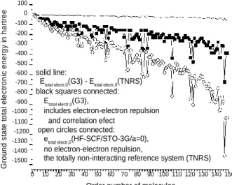
Ground state total electronic energy in hartree
One other expression stemming from the variation principle has to be emphasized: The S0 from HF- SCF/basis/a=1 for Eq.1 is energetically better than Y0 from HF-SCF/basis/a=0, when one uses this Y0 for Eq.1 at a=1, that is,
Eelectr,0 = <S0|H(a=1)|S0> + Ecorr < <S0|H(a=1)|S0> ≤ eelectr,0 + (N(N-1)/2)<Y0|r12-1|Y0>, (10) where the equality may come up when small e.g., STO-3G basis set is used. The error (correlation energy) of the middle part in Eq.10 with S0 stems from the fact that 0 is approximated with incorrect wave function form, namely with single determinant S0; but at least the LCAO coefficients vary slowly between Y0(a=0) and S0(a=1). (Again, the LCAO parameters in correct functional form Y0 come from solving Eq.1 at a=0 numerically, while in the incorrect functional form S0 the LCAO parameters come from the energy minimization of <S0|H(a=1)|S0> for Eq.1, restricted by the known ortho-normalization for MOs in both.)
100 0 -100 -200 -300 -400 -500
-600 solid line:
-700 Etotal electr,0(G3) - Etotal electr,0(TNRS) -800 black squares connected:
-900 Etotal electr,0(G3),
-1000 includes electron-electron repulsion -1100 and correlation efect
-1200 open circles connected:
-1300 etotal electr,0(HF-SCF/STO-3G/a=0), -1400 no electron-electron repulsion,
-1500 the totally non-interacting reference system (TNRS)
0 10 20 30 40 50 60 70 80 90 100 110 120 130 140 150 Order number of molecules
FIGURE 1. The 150 neutral test molecules from the G3 set are chosen as increasing N, e.g. 1: H2, 10: OH radical, 20: CO, 30: C2H5 radical, 40:
allene (C3H4), 50: aziridine, 60:
(CH3)2NH, 70: glyoxal, 80: acetone, 90: methyl ethyl ether, 100: twist C5H10, 110: n-pentane, 120: N-methyl pyrrole, 130: 3-methyl pentane, 140:
CH3CH2CH(CH3)NO2,147: C2F6, 148:
naphthalene,149: azulene (C10H8).
The shape of the curve itself has no particular mean, the important message is that the two curves (black squares and open circles) run together like the same fingerprint.
The related curve for open circles in Fig.1 with larger 6-31G** basis set would yield lower energy values by about 2% (basis set error improvement), and would be almost at the same position for eyes, not plotted. Solid line is the deviation Etotal electr,0(G3) - Etotal electr,0(TNRS) via first approximation in Eq.3 which brings the open circle values (a=0 in Eq.1 with small basis set error) remarkably back to black square ones (a=1 in Eq.1 with G3 estimation), it is also the approximate error of the (1,1) element of the CI matrix in Eq.5.
ACKNOWLEDGMENTS
Financial and emotional support for this research from OTKA-K 2015-115733 and 2016-119358 are kindly acknowledged. The subject has been presented in ICNAAM_2018_82, Greece, Rhodes.
REFERENCES
1.: A.Szabo, N.S.Ostlund: Modern Quantum Chemistry: Introduction to Advanced Electronic Structure Theory, 1982, McMillan, New York.
2.: Z.Peng, S.Kristyan, A.Kuppermann, J.Wright, Physical Review A, 52, 1005-1023 (1995).
3.: S.Kristyan, P.Pulay, Chemical Physics Letters, 229, 175-180 (1994).
4.: S.Kristyan, Computational and Theoretical Chemistry, 975, 20-23 (2011).
5: S.Kristyan: Eigenvalue equations from the field of theoretical chemistry and correlation calculations, arXiv:1709.07352 [physics.chem-ph]