Global Dynamics of a Novel Delayed Logistic Equation Arising from Cell Biology

https://doi.org/10.1007/s00332-019-09577-w

Global Dynamics of a Novel Delayed Logistic Equation Arising from Cell Biology

Ruth E. Baker¹·Gergely Röst^1,2

Received: 9 January 2019 / Accepted: 22 August 2019 / Published online: 31 August 2019

© The Author(s) 2019

Abstract

The delayed logistic equation (also known as Hutchinson’s equation or Wright’s equation) was originally introduced to explain oscillatory phenomena in ecological dynamics. While it motivated the development of a large number of mathematical tools in the study of nonlinear delay differential equations, it also received criticism from modellers because of the lack of a mechanistic biological derivation and interpretation.

Here, we propose a new delayed logistic equation, which has clear biological under- pinning coming from cell population modelling. This nonlinear differential equation includes terms with discrete and distributed delays. The global dynamics is completely described, and it is proven that all feasible non-trivial solutions converge to the posi- tive equilibrium. The main tools of the proof rely on persistence theory, comparison principles and anL²-perturbation technique. Using local invariant manifolds, a unique heteroclinic orbit is constructed that connects the unstable zero and the stable posi- tive equilibrium, and we show that these three complete orbits constitute the global attractor of the system. Despite global attractivity, the dynamics is not trivial as we can observe long-lasting transient oscillatory patterns of various shapes. We also discuss the biological implications of these findings and their relations to other logistic-type models of growth with delays.

Keywords Cell population·Logistic growth·Go-or-grow models·Time delay· Global attractor·Stability·Long transient

Mathematics Subject Classification 92D25·34K20

Communicated by Dr. Anthony Bloch.

B

1 Mathematical Institute, University of Oxford, Oxford, UK 2 Bolyai Institute, University of Szeged, Szeged, Hungary

1 Introduction

The well-known logistic differential equationN(t)=r N(t) (1−N(t)/K)was pro- posed by Verhulst in 1838 to resolve the Malthusian dilemma of unbounded growth (Bacaër2011). Here,N(t)represents the population density at timet,ris referred to as the intrinsic growth rate, andKas the carrying capacity. Generally, such saturating population growth can be achieved by assuming that an increase in the population size leads to a decrease in fertility or an increase in mortality. This is reasonable when resources are limited: if the population size exceeds some critical level, the habi- tat cannot support further growth. The logistic equation has seen widespread use in modelling studies across biology with applications in single bacteria, cell and animal populations, and also interacting populations, cancer and infectious diseases.

In the framework of the logistic ordinary differential equation, the population always converges to a stable steady state. However, in the context of ecology, oscillatory behaviours have also been observed, even in the absence of external periodic forcing.

For example, in Daphnia populations, oscillations are possible because the fertility of females depends not merely on the actual population density, but also on the past densities to which it has been exposed. This motivated Hutchinson in (1948) to propose the delayed logistic equation (also known as Hutchinson’s equation)

v(t)=αv(t)[1−v(t−τ)], (1) where we have normalized the carrying capacity to unity (by settingv(t)=N(t)/K) and introduced the time delayτ >0. Interestingly, independent of Hutchinson, in 1955 Wright (1955), motivated by an unpublished note of Lord Cherwell about a heuristic approach to the density of prime numbers, studied in detail the delay differential equation

u(t)= −αu(t−τ)[1+u(t)]. (2) Wright’s equation is an equivalent form of the delayed logistic equation, established via the change of variablesu(t)=v(t)−1.

Since the delayed logistic equation exhibits stable periodic solutions whenever ατ > π/2, it is very tempting to use this modification of the logistic ordinary differ- ential equation to explain observed biological oscillations. One example is the work of May fitting the delayed logistic equation to the empirical data of oscillatory blowfly populations from Nicholson’s experiments (May1973). However, the use of Hutchin- son’s delayed logistic equation received criticisms from biological modellers due to the lack of a mechanistic biological derivation (Geritz and Kisdi2012), the main objection being that it is not based on clearly defined birth and death terms, and the delay was inserted on a purely phenomenological basis. Indeed, in May’s work the parameters in the mathematical model did not directly correspond to any biological parameters.

Later, Gurney et al. (1980) proposed the equation

N(t)=a N(t−τ)e^{−bN(t−τ)}−μN(t), (3)

which is known today as Nicholson’s blowfly equation. It is structurally different from the delayed logistic equation, and the terms have clear biological interpretation as the birth and mortality rates, while the delay represents the period between egg laying and hatching. Furthermore, in contrast to the delayed logistic equation, Nicholson’s blowfly equation can explain not only the appearance of cycling populations, but also the two bursts of reproductive activity per adult population cycle that appeared in Nicholson’s data.

Incorporating a delay in the growth term, Arino et al. (2006) derived an alternative formulation of the delayed logistic equation

N(t)= γ μN(t−τ)

μe^μτ+κ(e^μτ−1)N(t−τ)−μN(t)−κN(t)², (4) which has recently been extended to distributed delays (Lin et al.2018). This model behaves similarly to the classical logistic equation, in the sense that it cannot sustain periodic oscillations; however, large delays cause the extinction of the population.

In another recent work, Lindström studied chemostat models with time lag in the conversion of the substrate into biomass (Lindström2017) and obtained equations of logistic type with delays as a limiting case. Lindström’s equation shares the same dynamical properties as the alternative delayed logistic equation from Arino et al.

(2006), both generating a monotone semiflow, unlike Hutchinson’s equation.

In addition to these biological applications, the delayed logistic equation moti- vated the development of a large number of analytical and topological tools, including local and global Hopf bifurcation analysis for delay differential equations (Chow and Mallet-Paret 1977; Faria 2006; Hassard et al. 1981; Nussbaum 1975), asymptotic analysis Fowler (1982), 3/2-type stability criteria (Ivanov et al.2002; Wright1955) and the study of slowly oscillatory solutions (Lessard2010). The most famous related problem is Wright’s conjecture from 1955, which proposes global asymptotic stability in the delayed logistic equation forατ ≤π/2. This long-standing question has been resolved recently by combining analytical and computational tools (Bánhelyi et al.

2014; van den Berg and Jaquette2018). Moreover, many variants and generalizations of the delayed logistic equation have been studied in the mathematical literature, for instance equation including positive instantaneous feedback (Gy˝ori et al.2018), non- autonomous terms (Faria2006), neutral terms (Gopalsamy and Zhang1988), spatial diffusion (Zou2002) and multiple delays (Yan and Shi2017). Further examples are discussed in Kuang (1993), Liz (2014), Ruan (2006).

In this paper, we derive a novel type of delayed logistic equation, inspired by cell biology. Our equation includes both terms with and without delays, as well as with distributed delays. After presenting derivation of the model in Sect.2, we study its basic mathematical properties in Sect. 3, such as well-posedness, existence and stability of equilibria. The global dynamics is fully described in Sect.4, and we provide a complete description of the global attractor. While all non-trivial solutions converge to the positive equilibrium, the model exhibits long-lasting transient oscillations of various shapes; this phenomenon is discussed in Sect.5. Finally, we summarize our findings and discuss their implications for future research in Sect.6.

2 Derivation of the New Delayed Logistic Equation

We derive our new delayed logistic equation by considering the mean-field limit of a simplistic agent-based, on-lattice model that describes both cell motility and pro- liferation, and cell–cell interactions through the incorporation of volume exclusion.

More specifically, we assume that agents move and proliferate on ann-dimensional square lattice with spacingΔand length (in each direction)Δ, whereis an integer describing the number of lattice sites. A great interest in current medical research is to understand the roles of two particular phenotypes, namely “high proliferation-low migration” and “low proliferation-high migration”, in the progression of aggressive cancers (Noren et al.2016). Our model is designed to capture the “go or grow” hypoth- esis frequently acknowledged in the cancer literature (Farin et al.2006; Giese et al.

2003), which proposes that cell proliferation and migration are temporally exclusive events.

As such, we divide our agent population into two subpopulations, motile and pro- liferative. Each agent is assigned to a lattice site, from which it can move or proliferate into an adjacent site. If a motile agent attempts to move into a site that is already occupied, the movement event is aborted. Similarly, if a proliferative agent attempts to proliferate into a site that is already occupied, the proliferation event is aborted. Agents convert from being motile to proliferative at constant rater >0 per unit time. That is, rδt is the probability that a motile agent switches to become proliferative in the next infinitesimally small time intervalδt. Upon switching, agents remain immobile for a fixed timeτ >0 (representing the length of time taken for cells to progress through the cell cycle to division), and they then attempt to proliferate by placing a daughter agent into one of the nearest neighbour lattice sites. We assume that daughter agents are initially motile. After attempting proliferation, proliferative agents switch back to being motile. We assume that agents do not die, reflecting that malignant cells tend to evade apoptosis. The initial agent distribution is, on average, spatially uniform and is achieved by populating lattice sites uniformly at a given probability.

Following arguments presented in Baker and Simpson (2010) and closing the hierarchy of moment equations at the pair level (assuming that the occupancy of neighbouring lattice sites is independent), we can derive a system of delay differential equations that describe how the density of agents on the lattice evolves over time:

m(t)= −r m(t)+r m(t−τ)+r m(t−τ)

K −p(t)−m(t) K

, (5)

p(t)=r m(t)−r m(t−τ), (6)

wheremis the density of motile agents,pis the density of proliferative agents,K >0 is the number of sites on the lattice (one can think of the carrying capacity asK =ⁿ) anddenotes differentiation with respect tot.

This mean-field model can be obtained directly as well by the following biological modelling arguments. The equations encode the model assumption that motile agents become proliferative with per capita raterand stay in this proliferative phase for time τ, this is reflected by (6). Once the cell cycle is completed, proliferative cells switch

back to being motile cells again, that is the middle termr m(t −τ)in equation (5).

The last term of Eq. (5) is obtained as follows. As the time needed for cell division elapsed, a daughter agent is placed into a lattice site, but only if that site is empty, otherwise the proliferation event is cancelled. The probability that site is empty at time t (in the mean-field limit) is(K −p(t)−m(t)) /K, which is the number of empty sites(K−p(t)−m(t))divided by the total size Kof the cell space. At timet, such attempts of placing daughter cells occur with rater m(t−τ), since this is the rate cells converted from motile to proliferativeτ time ago. Hence, successfully completed cell proliferations occur at rater m(t −τ)

K−p(t)−m(t) K

, which is the increase in the mpopulation due to proliferation, since we assumed that daughter cells are initially motile. Let us note that since we assumed that there is no cell death in the model, there are no mortality terms in (5)–(6), and the term representing switching back frompto mis exactlyr m(t−τ).

System (5)–(6) can be rewritten as a scalar equation using the natural biological relation

p(t)= _t

t−τr m(s)ds,

that is, the proliferative cells at timetare exactly those who entered the proliferative subpopulation in the time interval[t−τ,t]. Using this relation in equation (5) gives

m(t)= −r m(t)+r m(t−τ)+r m(t−τ)

1− r K

_t

t−τm(s)ds−m(t) K

.

Next, we rescale the density withK by lettingm(t)˜ =m(t)/K,

˜

m(t)= −rm(t)˜ +rm(t˜ −τ)+rm(t˜ −τ)

1−r t

t−τm(s)˜ ds− ˜m(t)

,

and drop the tildes and rearrange to m(t)= −r m(t)+r m(t−τ)

2−r

_t

t−τm(s)ds−m(t)

. (7)

To complete the non-dimensionalization, we also rescale time by letting t˜ = t/τ andx(t˜)=m(t). Then, dx/dt˜=τm(t)and, moreover,m(t−τ)=m(τt˜−τ)= m(τ(t˜−1))=x(t˜−1). Noting that

_t

t−τm(s)ds=τ _t˜

˜ t−1

x(˜s)ds˜,

we can, again, drop the tildes, to arrive at the new delayed logistic equation:

dx

dt = −rτx(t)+rτx(t−1)

2−rτ _t

t−1

x(s)ds−x(t)

. (8)

3 Basic Mathematical Properties

With the notationρ =rτ >0, we now analyze the scalar differential equation with discrete and distributed delays

x(t)= −ρx(t)+ρx(t−1)

2−ρ _t

t−1

x(s)ds−x(t)

. (9)

LetC=C([−1,0],R)denote the Banach space of continuous real-valued functions on the interval[−1,0]equipped with the supremum norm. Then, equation (9) is of the formx(t)= f(xt), where the solution segmentxt ∈Cis defined by

xt(s):=x(t+s), s∈ [−1,0].

Then, the map f :C→ Ris given by f(φ)= −ρφ(0)+ρφ(−1)

2−ρ

0

−1

φ(s)ds−φ(0)

, (10)

and the initial data are specified by

x0=φ∈C. (11)

3.1 Well-Posedness

By a solution of Eqs. (9), (11), we mean a continuous functionx(t)on an interval [−1,A)with 0< A≤ ∞, which is differentiable on(0,A), satisfies Eq. (9) on(0,A) and also satisfies Eq. (11).

Lemma 3.1 For everyφ∈C, there exists a unique solution of the initial value prob- lem(9), (11)defined on an interval[−1,A)for some0 < A ≤ ∞that depends continuously on the initial data.

Proof Recall the standard existence and uniqueness theorem for functional differential equations (Smith2011). We shall verify that the local Lipschitz property holds for f, i.e. for anyM >0, there is anL >0 such that

|f(φ)− f(ψ)| ≤L||φ−ψ||, whenever||φ||<M, ||ψ||<M.

For a constantM >0, let||φ||<M and||ψ||<M, then we have the estimates

|f(φ)− f(ψ)| ≤ρ||φ−ψ|| +2ρ||φ−ψ|| +ρ φ(−1)

ρ

0

−1

φ(s)ds+φ(0)

−ψ(−1)

ρ ₀

−1ψ(s)ds+ψ(0)

≤3ρ||φ−ψ|| +ρ φ(−1)

ρ

0

−1

φ(s)ds+φ(0)

−ψ(−1)

ρ 0

−1

φ(s)ds+φ(0) +ρ

ψ(−1)

ρ ₀

−1

φ(s)ds+φ(0)

−ψ(−1)

ρ ₀

−1ψ(s)ds+ψ(0)

≤

3ρ+ρ²M+ρM+Mρ²+ρM

||φ−ψ||.

Hence,L =3ρ+M

2ρ²+2ρ is a valid Lipschitz constant. Existence, uniqueness and continuous dependence then follow from the general theory, c.f. Theorem 3.7 of

Smith (2011) and (Kuang1993, Chapter 2).

Due to biological constraints, we are interested only in non-negative solutions, i.e.

x0(s)≥0,s∈ [−1,0]. More specifically, we consider solutions withx0∈Ω, where Ω :=

φ∈C :φ(s)≥0 fors∈ [−1,0]andφ(0)+ρ ₀

−1φ(s)ds≤1

. (12)

This set in fact corresponds to the biologically feasible phase space since, for a solution withxt ∈Ω,

θ(t):=x(t)+ρ t

t−1

x(s)ds

represents the total cell density (accounting for all mobile and proliferating cells) that should, in the non-dimensional model, lie between zero and unity. We shall useΩ ⊂C, the set of biologically feasible states as our phase space, noting thatΩdepends on the parameterρ.

3.2 Positivity and Boundedness from Above

Lemma 3.2 The setΩis positively invariant.

Proof We claim that ifθ(0)≤1, thenθ(t)≤1 fort>0. Note that θ(t)= −ρx(t)+ρx(t−1)

2−ρ

t t−1

x(s)ds−x(t)

+ρx(t)−ρx(t−1),

which simplifies to

θ(t)=ρx(t−1)(1−θ(t)). (13)

Forw(t):=1−θ(t), we havew(t)= −θ(t)= −ρx(t−1)w(t), and hence, w(t)=w(0)exp

−ρ t

0

x(s−1)ds

≥0, (14)

wheneverw(0)≥0, or equivalentlyθ(0)≤1. We find that θ(t)=x(t)+ρ

t t−1

x(s)ds≤1,

holds if

x(0)+ρ ₀

−1

x(s)ds≤1.

The general positivity condition, i.e. thatxt ≥0 wheneverx0≥0, for system (9),(11) is thatxt ≥ 0 and x(t) = 0 implies f(xt) ≥ 0 (Smith 2011, Theorem 3.4). This clearly holds as forx(t)=0, we have f(xt)=ρx(t−1)(2−θ(t))≥ 0 following fromxt ≥ 0 andθ(t)≤ 1. Sincext ∈ Ω is equivalent toxt ≥ 0 andθ(t)≤ 1, we obtain thatΩ is positively invariant, and additionally the estimatex(t) <1 holds.

Consequently, solutions starting fromφ ∈ Ω exist globally, i.e. on the interval [−1,∞), with x_t^φ ∈ Ω for allt ≥ 0, where the notation x_t^φ emphasizes that the solution corresponds to initial dataφ, i.e.x0=φ.

3.3 Steady States and Their Stability

Theorem 3.1 Equation(9)has two steady states,x˚=0which is always unstable, and x_∗=1/(ρ+1)which is always locally asymptotically stable.

Proof Settingx=0, we obtain the steady-state equation 0= −ρx+ρx(2−ρx−x) , which has the solutions ˚x=0, andx_∗=1/(ρ+1).

Linearization of Eq. (9) aroundx=0 gives

x(t)= −ρx(t)+2ρx(t−1), with the characteristic equation

λ+ρ=2ρe^−λ,

which always has a positive real root, and hence, 0 is unstable.

Next, we look at the stability of the equilibriumx_∗. Using the definition in Eq. (10), we have

f(x_∗+φ)= −ρ(φ(0)+x_∗)+ρ(φ(−1)+x_∗)

×

2−ρ 0

−1

(φ(s)+x_∗)ds−(φ(0)+x_∗)

=L(φ)+g(φ),

which has linear part

L(φ)= −ρ

1+ 1

ρ+1

φ(0)+ρφ(−1)− ρ² ρ+1

₀

−1φ(s)ds, and

g(φ)=ρφ(−1)

−ρ ₀

−1

φ(s)ds−φ(0)

.

Clearly, lim_||φ||→0|g(φ)|/||φ|| =0, and hence, the linear variational equation is

y(t)= −ρ

1+ 1

ρ+1

y(t)+ρy(t−1)− ρ² ρ+1

_t

t−1

y(s)ds.

The exponential ansatzy(t)=e^λtgives the characteristic equation λ= −ρ

1+ 1

ρ+1

− ρ² ρ+1

_t

t−1

e^λ(s−t)ds+ρe^−λ, (15)

which becomes, after integration and rearranging, λ²= −ρ

1+ 1

ρ+1

λ− ρ²

ρ+1(1−e^−λ)+ρλe^−λ, providedλ=0. Note thatλ=0 is not a root of Eq. (15), otherwise

0= −ρ

1+ 1

ρ+1

− ρ²

ρ+1 +ρ= −ρ <0,

which is a contradiction. Therefore, we may write the characteristic equation as χ(λ)=P(λ)+Q(λ)e^−λ=0, (16)

with

P(λ)=λ²+ρ

1+ 1

ρ+1

λ+ ρ² ρ+1, Q(λ)= − ρ²

ρ+1 −ρλ.

We can factor the characteristic equation as χ(λ)=

λ+ ρ

ρ+1 λ+ρ−ρe^−λ =0, (17)

which demonstrates that we always have the real rootλ= −ρ/(ρ+1) <0. The other roots are the roots ofλ+ρ−ρe^−λ=0. This is a well-known type of characteristic equation of the formλ=A+Be^−τλ, see, for example, Chapter 4.5 of Smith (2011).

However, we are on the stability boundary of this equation given thatλ=0 is a root (which is, as we established, not a root of the original characteristic equation (15)).

We can quickly show that all other roots have imaginary parts less than zero: assuming a root withλ≥0 butλ=0, we have

ρ <|λ+ρ| = |ρe^−λ| ≤ρ,

which is a contradiction. Therefore, the equilibriumx_∗is locally asymptotically stable.

4 Global Dynamics 4.1 Persistence

Theorem 4.1 Equation(9)is strongly uniformly persistent; that is, there exists aδ >0, independent of the initial data, such that for any solution x^φ(t)withφ(0) >0,

lim inf

t→∞ x(t)≥δ.

Proof Let

g(ψ)=ρψ(−1)

2−ψ(0)−ρ ₀

−1ψ(s)ds

, (18)

then Eq. (9) can be written as

x(t)= −ρx(t)+g(xt).

From the variation in constants formula, for anyσ > ω >0 we find x(σ)=e^{−ρ(σ−ω)}

x(ω)+

_σ

ω e^ρ(s−ω)g(xs)ds

.

We use the notationx_∞ =lim inft→∞x(t), andx^φ denotes a specific solution with initial functionφ. Assume the contrary of the statement of the theorem. Then, there is a sequenceφn, such that limn→∞x_∞^φn =0. Letq ∈(0,1)such thatq⁴>1/2 (any q >0.841 is just fine). Then, there is aTn→ ∞, such thatx^φn(t)∈ [q x^φ_∞ⁿ,1]for all t >Tn−1. Furthermore, there is atn>Tn+nsuch thatx^φn(tn)∈ [q x_∞^φn,q⁻¹x^φ_∞ⁿ].

For the particular casex=x^φn, σ =tnandω=Tn, the variation in constants formula gives

x^φn(tn)=e^{−ρ(tn−Tn)}

x^φn(Tn)+ _tn

T_n

e^ρ(s−Tn)g x_s^φn ds

.

Using the integral mean value theorem, there is anηn∈ [Tn,tn], such that e^−ρtn

_tn

Tn

e^ρsg

x^φ_sⁿ ds=e^−ρtng

x_η^φ_nⁿ

tn

Tn

e^ρsds=g

x_η^φ_nⁿ ρ⁻¹

1−e^ρ(Tn−tn) .

Then, we have the relation

x^φn(tn)=e^{−ρ(tn−Tn)}x^φn(Tn)+g

x_η^φ_nⁿ ρ⁻¹

1−e^ρ(Tn−tn)

. (19)

Since x^φn(tn) → 0,e^{−ρ(tn−Tn)}x^φn(Tn) → 0 and

1−e^Tn−tn → 1 as n → ∞, necessarilyg

x^φ_ηnⁿ

→ 0 as well asn → ∞. Sincex_η^φ_nⁿ ∈ Ω,we haveg

x_η^φ_nⁿ ≥ ρx_η^φ_nⁿ(−1), and hence,x^φn(ηn−1)→0 as well asn→ ∞.

Next, we claim that

2−x^φn(ηn)−ρ 0

−1

x^φn(ηn+s)ds

→2 asn→ ∞. (20)

From the inequalityx(t)≥ −ρx(t), we find thatx^φn(ηn+s)≤e^ρx^φn(ηn−1)for s∈ [−1,0]. Hence,

x^φn(ηn)+ρ ₀

−1

x^φn(ηn+s)ds≤e^ρx^φn(ηn−1)(1+ρ),

and the right-hand side is already shown to converge to zero, and thus, (20) holds. For sufficiently largen, we have the estimateg

x_η^φ_nⁿ

≥2qρx_η^φnⁿ(−1)≥2qρq x_∞^φn (where the first inequality follows from (18) and (20)) and

1−e^ρ(Tn−tn) > q, therefore, from equation (19) we obtain

q⁻¹x_∞^φn ≥x^φn(tn)≥2q³x^φ_∞ⁿ.

We find 1≥2q⁴, which contradicts the choice ofq.

4.2 A Crucial Convergence Property

Theorem 4.2 For all positive solutions, we have

tlim→∞

x(t)+ρ t

t−1

x(s)ds

=1.

Proof This follows from the standard comparison principle, since for largetwe have 1>x(t−1) > δ/2>0, and by Eq. (13), we see thatθ(t)is squeezed betweenθ(t) andθ(t¯ ), which are the solutions of

θ(t)=ρδ

2(1−θ(t)), and

θ¯(t)=ρ(1− ¯θ(t)),

withθ(0)= ¯θ(0)=θ(0) >0, each converging to unity.

4.3 Global Asymptotic Stability

Theorem 4.3 All positive solutions of Eq.(9)inΩconverge to the positive equilibrium.

Proof First, we recall the following theorem from Gy˝ori and Pituk (1995):

Theorem A (Gy˝ori-Pituk)Consider

x(t)=(a0+a(t))x(t)+(b0+b(t))x(t−τ),

where a0,b0 ∈ R, τ > 0 are constants and a,b : [0,∞) → R are continuous functions. Let the following assumptions be satisfied:

(i) λ =a0+b0e^−λτ has a unique rootλ0with the largest real part, and this root λ0is real and simple;

(ii) a(t)→0, b(t)→0as t → ∞; (iii) _∞

0 a²(t)dt<∞,_∞

0 b²(t)dt<∞; (iv) _∞

0

τa(t)−_t

t−τa(s)dsdt<∞,_∞

0

τb(t)−_t

t−τb(s)dsdt<∞.

Then, every solution x(t)satisfies x(t)=exp

t 0

λ(s)ds

(ξ+o(1)) , t → ∞,

where

λ(t)=λ0+

1+b0τe^{−λ0τ −1}

a(t)+e^−λ0τb(t) ,

andξ =ξ(x)is a constant depending on the solution x.

Fix someψ∈Ω, and letx^ψ(t)be the corresponding solution with w^ψ(t)=1−x^ψ(t)−ρ

_t

t−τx^ψ(s)ds=w(0)exp

−ρ _t

0

x^ψ(s−1)ds

,(21)

where the last equality was given in Eq. (14). Now consider the equation z(t)= −ρz(t)+ρz(t−1)

1+w^ψ(t) . (22)

We apply TheoremAand check all the conditions, where we havea0= −ρ,b0=ρ, τ = 1, a(t) = 0 and b(t) = ρw^ψ(t). The conditions with a(t)are trivial, and the conditions withb(t)follow from the combination of persistence and Eq. (21) as follows, sincewis exponentially convergent.

(i) λ= −ρ+ρe^−λhas a unique rootλ0with the largest real part, and this rootλ0

is real and simple (in factλ0=0).

(ii) To see thatw^ψ(t)→0 ast → ∞, we can use Theorem 4.1: there is aδ >0 and aT such thatx(t) > δfort>T −1. From equation (21), we find

w^ψ(t)=w(0)exp

−ρ _T

0

x^ψ(s−1)ds

exp

−ρ _t

T

x^ψ(s−1)ds

< w(0)exp

−ρ T

0

x^ψ(s−1)ds

e^{−ρδ(t−T)}, (23) or

w^ψ(t) < K e^−ρδt, K =w(0)exp

−ρ T

0

x^ψ(s−1)ds

e^rδT. (24) (iii) The estimate in Eq. (24) shows that

_∞

0

w^ψ(t)² dt <K² _∞

0

e^−2ρδtdt= K² 2ρδ <∞.

(iv) From the estimate in Eq. (24), we also find that _∞

0

w^ψ(t)− _t

t−1

w^ψ(s)ds dt <

_∞

0

w^ψ(t)dt+ _∞

0

_t

t−1

w^ψ(s)dsdt <∞.

As a result,

λ(t)=(1+ρ)⁻¹ρw^ψ(t),

and all the conditions of Theorem A hold. Thus, every solutionz(t)satisfies z(t)=exp

(1+ρ)⁻¹ρ t

0

w^ψ(s)ds

(ξ+o(1)), t → ∞.

Now notice that a solutionx(t)of Eq. (9) with initial functionψis also a solution of Eq. (22), and hence, it converges to a constant. In view of Theorem4.1, this constant

can only be the positive equilibrium.

4.4 The Global Attractor

Denote byΦ^Ω the semiflow onΩ generated by (9). We say that a subset ofΩis the global attractor ofΦ^Ω, if it is compact, invariant and attracts each bounded subset of Ω.

Theorem 4.4 The global attractorAconsists of the two equilibria and a heteroclinic orbit connecting the two.

Proof First, we demonstrate that the global attractorAofΦ^Ωexists. From the positive invariance of the bounded setΩ, this semiflow generated by the equation onΩis point dissipative. It follows from the Arzelà-Ascoli theorem that the solution operatorsΦ_t^Ω are completely continuous fort ≥1; then, by applying Theorem 3.4.8 of Hale (1988), the compact global attractor exists.

The two equilibria are part of the global attractor. Next, we show that there exists a unique heteroclinic orbit inΩ connecting ˚x =0 and the positive equilibrium,x_∗. Recall that the characteristic equation of the linearization at ˚x=0 isλ+ρ=2ρe^−λ, which has a single positive root λ0. The other roots form a sequence of complex conjugate pairs(λj,λ¯j)withλj+1 < λj < λ0for all integers j ≥ 1. We refer to Chapter XI of Diekmann et al. (2012) for a complete analysis of the characteristic equation of the formz−α−βe^−z, in particular Fig. XI.1. in Diekmann et al. (2012) which summarizes its properties. Our equation is a special case withα= −ρ,β =2ρ. There is aγ >0 such thatλ0> γ >λj for all j ≥1, and there is ak∈Nsuch thatλk>0 andλk+1≤0, where the point(−ρ,2ρ)lies between the curvesC⁻_k andC_k⁻₊₁on the(α, β)-plane, given by

C⁻_j =

(α, β)=νcosν sinν ,− ν

sinν

: ν∈((2j−1)π,2jπ) .

The intersections ofC⁻_j and the half-line(−ρ,2ρ)(ρ >0) are determined by cosν= 1/2, and thus,ν = 2jπ −π/3, sinν = −√

3/2 and the intersection is given by ρ =ρj =(2jπ −π/3)/√

3.Hence,kis either zero or the largest positive integer such thatρ > ρk.

Considering the leading real root, the corresponding eigenfunction is given by χ0(s):=e^λ0s,s∈ [−1,0].The phase spaceCcan be decomposed asC=P0⊕Pk⊕Q, where the functionχ0 ∈C spans the linear eigenspaceP0:= {cχ0 : c∈ R}.Pk is a 2k-dimensional eigenspace corresponding to{λj : j =1, . . . ,k}. Ifλ0is the only eigenvalue with positive real part, thenPk = ∅. There is anε >0 such thatλk> ε.

Qcorresponds to the remaining part of the spectrum.

In what follows, we use local invariant manifold theorems for semiflows in Banach spaces, for the details see Faria et al. (2002) and Krisztin et al. (1999). Accordingly, there exist open neighbourhoodsN0,Nk,M of 0 inP0,Pk,Q, respectively, andC¹- mapsw0 : N0 → Pk ⊕ Q,wu : N0⊕ Nk → Q with range in Nk ⊕M and M, respectively, such thatw0(0) = 0, Dw0(0) =0,wu(0)= 0, Dwu(0)= 0; where Ddenotes the Fréchet derivative. Then, theγ-unstable set of the equilibrium ˚x =0, namely

W0(0):= {φ∈ N0+Nk+M :there is a trajectoryzt,t ∈Rwithz0=φ, zt ∈ N0+N1whent ≤0 andz(t)e^−γt →0 ast → −∞

, (25) coincides with the graph

W0:= {φ+w0(φ):φ∈ N0}.

Furthermore, the unstable set of the equilibrium ˚x=0

Wu(0):= {φ∈N0+Nk+M :there is a trajectoryzt,t ∈Rwithz0=φ, zt ∈N0+N1whent ≤0 andz(t)e^−εt →0 ast→ −∞

, (26) coincides with the graph

Wu:= {φ+wu(φ):φ∈N0+Nk}.

For anyφ ∈ N0, there is a c ∈ Rsuch thatφ = cχ0. We have||χ0|| = 1 and χ0(t)≥e^−λ0 >0 for allt∈ [−1,0]. It follows fromDw(0)=0 that

||φ||→lim0

||w(φ)||

||φ|| =0, φ∈ N0, which means

clim→0

||w(cχ0)||

|c| =0.

Therefore, there exists a c0 > 0 such that ||w(cχ0)||/|c| < e^−λ/2 whenever c ∈ (0,c0), or equivalently||w(cχ0)||<ce^−λ/2. We may assume thatc0<1/(2(1+ρ)).

Then,

min{cχ0(t)+w(cχ0)(t):t∈ [−1,0], c∈(0,c0)} ≥ce^−λ−c

2e^−λ= c

2e^−λ>0,

and

cχ0(0)+w(cχ0)(0)+r ₀

−1

{cχ0(s)+w(cχ0)(s)}ds≤(1+ρ)(c+ ||w(cχ0)||)

<2c0(1+ρ)

<1, and thus,

φc:=cχ0+w(cχ0)∈W0∩Ωfor allc∈(0,c0). (27) The unstable setW0(0)intersectsΩ, and for any functionφcof this intersection, there is a complete solution x(t) : R → R⁺₀ such that x0 = φc and xt → 0 as t → −∞. Fix such acand the corresponding solutionx(t). By the positive invariance of Ω, xt ∈ Ω for all t ≥ 0. By the negative invariance of W0(0), xt ∈ W0(0) for all t ≤ 0. Consider at˜ < 0, then x_t˜ ∈ W0(0); thus, there is a c˜ such that x_˜t = ˜cχ0+w(cχ˜ 0). SinceW0(0)is one dimension, fromx0 = φc andxt → 0 as t → −∞it follows thatc˜∈(0,c)⊂(0,c0); thus, from (27) we find thatx_t˜∈Ω. We have proved the existence of a heteroclinic orbit completely inΩ connecting the two equilibria.

For uniqueness, consider the unstable manifoldWu(0). Any solution on the set Wu(0)\W0(0)oscillates about 0 as t → −∞, and hence, it cannot be a positive heteroclinic solution. Denote the unique heteroclinic orbit inΩ byH. We claim that Hand the two equilibria constitute the global attractor, otherwise there are further complete orbits inΩ. Assume there is aψ ∈ Ω which is on such a complete orbit Γ ⊂Ω, soψ=0,ψ=x_∗andψ /∈H. Then, itsα-limit setα(ψ)andω-limit setω(ψ) are non-empty, compact and invariant. In particular, by Theorem4.3,ω(ψ)= {x_∗}. If α(ψ)= {x˚}, thenΓ is a connecting orbit coinciding withH. Hence, we may assume that there is aφ=0 such thatφ∈α(ψ). Then,x_t^φ→x_∗ast → ∞, sox_∗∈α(ψ)as well. But this contradicts the stability ofx_∗. Thus, the global attractor does not contain

any other orbit, andA= {x} ∪ {x˚ _∗} ∪H.

5 Numerical Simulations and Metastability

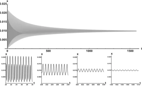
Representative numerical simulations of solutions of Eq. (9) are plotted in Fig.1, with initial functionφ(t)=0.005(cos(10t)+1)and parameter valuesρ=50,120,190.

To avoid numerical issues with representing the integral term, for the numerical simu- lations we used the system version of the model that includes only constant delay. As we can see in Fig.1, in a short time interval of length 10, the solutions appear to be periodic, with their periods approximately equal to the delay, despite the fact that we proved in Theorem4.3that all non-trivial solutions converge to the positive equilib- rium. Indeed, viewing the solution on a larger time scale in Fig.2, we can see that the solution is in fact not periodic; however, the convergence is very slow. This is a situa- tion that is sometimes called metastability. Paraphrasing (Holmes2012), metastability

190 192 194 196 198 200t

0.015 0.020 0.025

x

190 192 194 196 198 200t

0.005 0.010 0.015

x

190 192 194 196 198 200t

0.002 0.004 0.006 0.008 0.010 0.012x

Fig. 1 Representative solutions that appear periodic over short time scales. From left to right,ρ = 50,120,190 withφ(t)=0.005(cos(10t)+1)

0 500 1000 1500 t

0.005 0.010 0.015 0.020 0.025x

20 22 24 26 28 30t

0.005 0.010 0.015 0.020x

220 222 224 226 228 230t

0.005 0.010 0.015 0.020x

820 822 824 826 828 830t

0.005 0.010 0.015 0.020x

1400 1402 1404 1406 1408 1410t

0.005 0.010 0.015 0.020x

Fig. 2 Top: envelope of the solution with initial functionφ(t)=0.005(cos(10t)+1)andρ=100, showing slow convergence to the positive equilibrium. Bottom: snapshots of the same solution over different time intervals

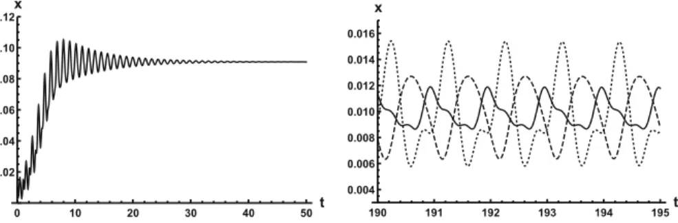
refers to a situation when something appears not to change on short time scales, while it changes after a sufficiently long period of time. Such phenomena are common in boundary value problems of partial differential equations, and metastability has been observed for delay differential equations as well, see, for example, Erneux (2009), Grotta-Ragazzo et al. (2010). Long-lasting transient oscillations have been reported in Morozov et al. (2016) for a scalar differential equation with a constant delay. It is interesting to see that Eq. (9) can exhibit rapid convergence for smallρand oscillatory patterns of various shapes for largerρ, as illustrated in Fig.3where solutions are plot- ted with different initial functions. Nevertheless, for such largeρ, these oscillations inxwill be very small compared to the total cell density which converges to one.

Since the long-lasting transient oscillations emerge for largeρ, to gain some under- standing of this phenomenon, we look at our model from the point of view of singular perturbations, lettingρ → ∞. In Eq. (9), let us divide byρ². For largeρ, we use the notationε=1/ρ, and then, we have

0 10 20 30 40 50t 0.02

0.04 0.06 0.08 0.10 0.12x

190 191 192 193 194 195t

0.004 0.006 0.008 0.010 0.012 0.014 0.016 x

Fig. 3 Left: convergence forρ =10 with initial functionφ(t) =0.005(cos(10t)+1). Right: various periodic patterns forρ = 100, emerging from initial functionsφ(t) = 0.005(cos(10t)+1)(dotted), φ(t)=0.005(cos(20t)+1)(solid),φ(t)=0.005(cos(10t⁴)+1)(dashed)

ε²x(t)=ε[−x(t)+2x(t−1)−x(t−1)x(t)]−x(t−1) _t

t−1

x(s)ds. (28) Settingε=0, we obtain the singular perturbation

0=x(t−1) _t

t−1

x(s)ds.

Besides x ≡ 0, any periodic function with unit period that is on average zero is a solution of this equation. While the singular limit is an equation from a different class, and its periodic solutions do not have non-negativity that we require for the differential equation, the behaviour of this singular limit may be a hint as to why we see long-lasting transient oscillations with a variety of shapes for largeρ.

In addition, we can look at the singular perturbation of the characteristic equation:

Eq. (17) can be written as λ²+ρ

1+ 1

ρ+1

λ+ ρ² ρ+1 =

ρ² ρ+1 +ρλ

e^−λ.

Multiplying by(ρ+1)/ρ², we have λ²ρ+1

ρ² +ρ+2

ρ λ+1=

1+λρ+1 ρ

e^−λ,

which is

λ²(ε²+ε)+(1+2ε)λ+1=(1+λ(1+2ε))e^−λ,

with the notationε=1/ρ. Settingε=0, we obtain the singular perturbation λ+1=(1+λ)e^−λ.

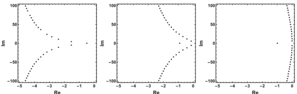
Fig. 4 Characteristic roots of (15) on the complex plane forρ=1,10,100. Asρ→ ∞, characteristic roots converge towards the imaginary axis

The roots of this equation satisfy either λ = −1 or e^−λ = 1, having the purely imaginary roots i = 2kπ,k ∈ Z. Indeed, as we increase ρ, we can see that all complex roots line up along the imaginary axis, see Fig.4.

6 Discussion

The delayed logistic equation has received much attention in past decades in the anal- ysis of nonlinear delay differential equations. However, its biological validity has been questioned, despite the fact that it was introduced by Hutchinson to explain observations of oscillatory behaviour in ecological systems. Here, we introduced a new logistic-type delay differential equation, derived from the go-or-grow hypothe- sis which has been observed for some types of cancer cells. The equation naturally includes a product of delayed and non-delayed terms, as well as both discrete and distributed delays. Detailed mathematical analysis reveals that all nonzero solutions converge to the stable positive equilibrium. For an alternative formulation of the delayed logistic equation (Arino et al. 2006), the authors also concluded that, as opposed to Hutchinson’s equation, sustained oscillations were not possible and solu- tions settled at an equilibrium. In some sense, the dynamical behaviour of our model is in-between these two extremes. While we have proved that all positive solutions are attracted to the positive equilibrium, for a range of parameters the convergence is so slow that, on a biologically realistic time scale, solutions may appear periodic. These long-lasting transient patterns can have various shapes, as shown in Fig.1, and these shapes also change in time (see Fig.2).

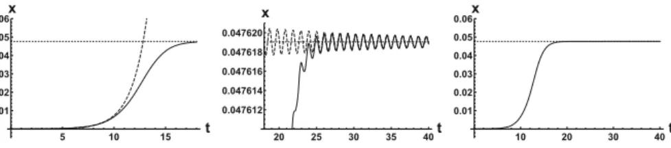
We have also fully described the global attractor as the union of the two equilibria and a unique connecting orbit. This heteroclinic solution is depicted in Fig.5when ρ=20. In this case, the leading real eigenvalue at zero isλ≈0.66, while the leading pair of eigenvalues at the positive equilibrium areλ≈ −0.04±6i. We can numerically observe how the solution is aligned to the leading eigenspaces of the linearizations near the two equilibria.

Our model is based on the commonly invoked modelling assumption that prolifer- ating cells abort proliferation when placement of a daughter cell is not possible due to spatial crowding constraints. However, there are other potential models of crowding-