Attractiveness and stability for Riemann–Liouville fractional systems

Attractiveness and stability for Riemann–Liouville fractional systems

Javier A. Gallegos

and Manuel A. Duarte-Mermoud

1Department of Electrical Engineering, University of Chile, Av. Tupper 2007, Santiago, Chile

2Advanced Mining Technology Center, University of Chile, Av. Tupper 2007, Santiago, Chile

Received 27 January 2018, appeared 29 August 2018 Communicated by Paul Eloe

Abstract. We propose a novel approach to study the asymptotic behavior of solutions to Riemann–Liouville (RL) fractional equations. It is shown that the standard Lyapunov approach is not suited and an extension employing two (pseudo) state spaces is needed.

Theorems of Lyapunov and LaSalle type for general multi-order (commensurate or non-commensurate) nonlinear RL systems are stated. It is shown that stability and passivity concepts are thus well defined and can be employed in L²-control. Main applications provide convergence conditions for linear time-varying and nonlinear RL systems having the latter a linear part plus a Lipschitz term. Finally, computational realizations of RL systems, as well as relationships with Caputo fractional systems, are proposed.

Keywords: fractional differential equations, Riemann–Liouville derivative, stability, at- tractiveness, multi-order, nonlinear systems.

2010 Mathematics Subject Classification: 34K37, 34D05, 34D45.

1 Introduction

The study of asymptotic properties of integer order systems have been greatly developed through the use of the Lyapunov method and the corresponding stability notions [14, Chap- ter 3]. The asymptotic stability of equilibrium points, in the Lyapunov sense, has become the main goal in control applications. Seemingly different techniques as passivity [14, Chap- ter 10] and input-output stability [14, Chapter 6], have deep connections with the Lyapunov functions.

Fractional systems have attracted the attention of researchers due to their non-local prop- erties, which allow to model complex phenomena [12,13]. In particular, RL systems present interesting mathematical challenges due to their singularities at the initial time (see [3] for the study of positive solutions). However, the Lyapunov theory has been mainly developed for Caputo fractional systems [6,10], since the formulation for RL fractional order systems present, as we will see in Section 2, an obstacle related to the initial conditions, that has remained un- noticed in the main papers on the subject [17,19]. Alternative methods like the Gronwall

BCorresponding author. Email: jgallego@ing.uchile.cl

inequality and the Barbalat lemma have limited applicability in fractional systems [7,11]. In- tegral equation approaches posit restrictive conditions for asymptotic stability (e.g. complete positive kernels [4]).

We aim to develop a Lyapunov approach to study asymptotic properties of RL systems. It involves the definition of suited stability and passivity concepts, the introduction of Lyapunov- like theorems and the illustration of their applicability. Our underlying objective is to show that RL systems have as good properties as the Caputo systems – which have become perva- sive in the literature – even in simulation aspects. Moreover, we show that multi-order systems (where each equation can have a different derivation order) can be easier to deal with RL than Caputo derivative.

In Section 3, we establish asymptotic results for RL systems, taking as a model the theory of Lyapunov functions. Specifically, similar results to Lyapunov, LaSalle and passivity theorems for mixed or multi-order nonlinear RL systems (also called non-commensurate) are obtained, which are contributions to the revised literature (cf. the recent work [21] where the systems are commensurate and restricted to a specific class of nonlinearity). Though the Lyapunov theory is powerful in many ways, it has the weakness that the Lyapunov function is not explicit from the equations and has to be constructed. In most of the cases, however, a quadratic function is enough. It turns out that quadratic functions are also effective for RL systems due to a quadratic inequality recently stated [2,17].

In Section 4, we provide main applications of our approach finding conditions for con- vergence of fractional time-varying linear and nonlinear systems. Finally, in Section 5, we propose a realization of RL systems based on standard software and relationships among Caputo and RL systems.

2 Preliminaries

In this section, we examine stability notions and relevant features of RL systems. The central concept in fractional calculus is the Riemann–Liouville fractional integral. For a function

f :[0,T]→C, it is given by [15, eq. 2.1.1], I^αf(t):= [I^αf(·)](t):= ¹

Γ(α)

Z _t

0

(t−τ)^α−1f(τ)dτ, (2.1) whereα∈_R>0and, without loss of generality, the initial time of the fractional integral is fixed att=0. It is well defined for locally integrable functions and directly generalizes the Cauchy formula for repeated integration [7, Lemma 1.1].

The Riemann–Liouville fractional derivative of orderαis defined by [15, eq. 2.1.5]

RD^αf :=D^mI^m−αf, (2.2)

wherem = dαeand the Caputo derivative is given by ^CD^αf := I^m−αD^mf (see [7, §2, 3] for a formal definition).

The Riemann–Liouville systems for 0 < α ≤ 1 are defined by the following initial value problem

(RD^αx:= f(x,t)

lim_t→0⁺ I^1−αx(t) =b, (2.3) wherex(t), f(x(t),t)∈_Rⁿ for allt>0 andb∈_Rⁿ. The initial condition lim_t→0⁺ I^1−αx(t) =b implies that, wheneverα < _{1 and}b6=_0, x ∈ C[/ _0,T]_{for any} T > 0, i.e. it is not a continuous

function on [0,T]. Indeed, if x ∈ C[0,T], then xis bounded on [0,T]but a bounded function yields lim_t→0⁺ I^1−αx(t) = 0, since |I^1−αx(t)| ≤ [I^1−αC](t) = O(t^1−α) where C is a constant bound on x. The behavior of x around t = 0 is given by t^α−1 [7], whereby the solution necessarily satisfies lim_t→0⁺x(t) =±_∞.

The stability concept is central in system theory and is usually meaning the Lyapunov notion. It characterizes the dynamic behavior in a neighborhood of a given set, for a system of trajectories x(·). In its simpler version [14, Definition 3.2], it states that an equilibrium point xeis Lyapunov stable, if for everye>0 there exists aδ> 0 such that, ifkx(0)−xek<δ, then kx(t)−x_ek< efor all t≥0, wherek · kdenotes the Euclidean norm.

Not only x(0) = ±_∞ makes the above stability notion unsuited but also the very concept of an equilibrium point – a point xe ∈ _Rⁿ such that if a system starts at xe, x(t) ≡ xe for all t≥ 0 – is meaningless, since on the one hand lim_t→0⁺x(t) =±_∞and on the other, the initial condition is not specified in terms of x. In the same way, global boundedness of solutions cannot be stated, unless that it is defined after some timeT >0.

Like the Caputo derivative [1], RL derivative has the following property when 0<α≤1

RD^αx²(t)≤2x(t)^RD^αx(t) ∀t ≥0, (2.4) whenever x ∈ C[0,T]or x∈ C^β[0,T]:= {u: [0,T]→_R :|u(t)−u(t−h)|= O(h^β)uniformly for 0≤t−h< t≤ T}for any 1> β>α/2 [2]. In [17], inequality (2.4) was proved under the stronger requirement of continuous differentiability (since it is used integration by parts).

Both references for (2.4) posit unsuited conditions whenxis a nontrivial solution of an RL system, since it belongs at best to C(0,T][7]. However, from the proof in [2], we observe that (2.4) holds for every t > 0 whenever x ∈ C(0,T]. If f = f(·,·) is continuous and Lipschitz continuous in its first argument, then uniqueness C(0,T]solutions are obtained [9]. Note that in this step, the condition f(0,t)≡0 becomes necessary for attractiveness ofx =0. Hereafter, we assume that these condition are satisfied for system (2.3).

Inequality (2.4) can be extended in at least two relevant ways. By an induction argument (see details in [2]), it can be proved that

RD^αxⁿ(t)≤nx^n−1RD^αx(t) ∀t >0, (2.5) for any even natural number n and if x ≥ 0, for any odd natural number. Second, for the vector case and using the same (algebraic) reasoning as in [8], where it was deduced for the Caputo operator, one obtains for any P∈_R^n×n,P>0,

RD^α[x^TPx](t)≤2x^TP^RD^αx(t) ∀t>0, (2.6) where x(t)∈_Rⁿ for allt>0 andx^T is the transpose vector.

To end this section, we recall some results which will be referenced along the paper. The Mittag-Leffler function is defined as E_α,β(_z) _:= _∑^∞_k=0Γ( ^zk

αk+β) [7], where α,β > _{0 and z} ∈ _C.

The Lebesgue spaces are defined asL^p := f :R≥0 →_Rⁿ | R

R≥0kfk^p dx¹_p

<_∞ forp≥1,

whereR≥0denotes the set of nonnegative real numbers. The Barbalat lemma [14] is given as follows.

Lemma 2.1. If f(t) is a uniformly continuous function, such that lim_t→_∞Rt

0 f(τ)dτ exists and is finite, thenlimt→_∞ f(t) =0. In particular, if f(t)is uniformly continuous function and f ∈ L¹ then lim_t→_∞ f(t) =0.

Finally, LaSalle’s theorem [14] can be expressed as follows.

Theorem 2.2. Let f(x)be a locally Lipschitz function defined over a domain D ⊂_Rⁿ andΩ⊂D be a compact set such that solutions ofx˙ = f(x)starting inΩremain inΩ. Let V(x)be a continuously differentiable function defined over D such thatV˙(x) ≤ 0 in Ω. Let E be the set of all points in Ω whereV˙(x) =0. Then every solution starting inΩapproaches to E as t→_∞.

3 Main results

In this section, we propose two complementary but clearly differentiated approaches to deter- mine asymptotic properties of RL systems.

3.1 Attractiveness approach

Instead of asymptotic stability, this approach provides conditions for the attractiveness of x=0 and boundedness of the solutions after any finite time. The strength of this approach relies on the next theorem, which is an analog of the Lyapunov direct theorem [14, Theo- rem 3.1] or the fractional Lyapunov theorem for Caputo systems [10,16]. For it, we need some definitions. A functionV :Rⁿ→_Ris a positive definite function if it is nonnegative,V(x)6=₀ for all x 6= 0 and V(0) = 0. More generally, function V = V(t,x)is positive definite if there exist positive definite functionsW₁,W₂ : Rⁿ → _R≥0 such thatW₂(x) ≥ V(x,t) ≥ W₁(x) for everyt ≥_{0 and}x∈_Rⁿ_.

Theorem 3.1. Suppose that for system(2.3)there exists k>0and a positive definite function V(x,t) such that for any initial condition

RD^αV(x(t),t)≤ −kV(x(t),t) ∀t >0,∀x∈_Rⁿ. (3.1) Then, lim_t→_∞x(t) = 0, i.e. x = 0 is globally attractive and x remains bounded on [T,∞) for any T>0. If (3.1)holds for some initial conditions b∈ _Ω⊂_Rⁿ, the precedent statement is local.

Proof. Since the comparison principle holds for RL equations (see for instance [16, Remark 6.2]) andV ≥0, it is enough for the first claim to study (3.1) in the equality.

The equation ^RD^αy = −ky has y(t) = bt^α−1Eα,α(−kt^α) as the unique solution ([15, eq.

4.1.10], see [7] for uniqueness), where lim_t→0⁺ I^1−αy(t) =b. From [6, Proposition 4],y →0 as t→_∞. By comparison, 0≤V(x(t),t)≤y(t). Then,V(t)→0 ast→_∞. Hence,W₁(x(t))→0 which impliesx(t)→0 ast→_∞.

Since x ∈ C(0,T] for any T > 0 and x(t) → 0 as t → ∞, we conclude that x remains bounded on[T,∞).

Remark 3.2.

(i) Whenα < 1, and using (2.2), ^RD^αV ≤ 0 is equivalent to _dt^dI^1−αV ≤ 0. Hence, I^1−αV is nonnegative, decreasing function and then, it converges. IfV(t) =V(x(t)_,t)is uniformly continuous and differentiable, limt→_∞V(t) = 0 [11]. Thus, in contrast to α = 1 (see Theorem2.2), condition ^RD^αV ≤0 could be enough to guarantee attractiveness instead of (3.1).

(ii) Unlike Lyapunov functions, it is allowed lim_t→0⁺V(x(t)) = +∞, for radially unbounded functionVsuch as V(x) =x^Tx.

With positive definite functions based on terms of type x²ⁿ and inequality (2.6), Theo- rem 3.1 can be very useful to get asymptotic properties of RL systems, as illustrated in the following example.

Example 3.3. Consider the system

(RD^αx= −x+xy^Ty

RD^αy=−x^Txy−y, (3.2)

where x(t)∈_Rⁿ,y(t)∈_R^m for everyt ≥0. The polynomial character of the right-hand side of (3.2) assures the continuity required to apply inequality (2.6). Then,

(RD^αx^Tx ≤ −2x^Tx+2x^Txy^Ty

RD^αy^Ty≤ −2x^Txy^Ty−2y^Ty.

By defining 2V(x,y) =x^Tx+y^Ty, we have

RD^αV ≤ −x^Tx−y^Ty=−2V.

Therefore, by applying Theorem3.1, limt→_∞x(t) =limt→_∞y(t) =0.

Example3.3also shows a drawback of this approach, shared by the similar approach for Caputo systems [10]. If the first equation of (3.2) has derivation orderαand the secondβ6= α, there is not a clear positive definite function candidate, even for such a simple system. The next approach is intended to deal with these more general systems, by finding a common order which, as suggested by the defining equation (2.2), must be an integer number.

3.2 Lyapunov mixed order approach

This approach will be shown in the proof of the next theorem. For it, we need some definitions.

Consider the following system

RD^αix_i(t) = f_i(x₁, . . . ,xn,t) (3.3) where 0 < α_i ≤ 1, x_i(t) : R≥0 → _R, f_i : Rⁿ×_R≥0 → _R and the initial conditions are given by lim_t→0⁺ I^1−αix_i(t) = b_i ∈_Rfori∈ {_{1, . . . ,}n}_{. Let}x := (x₁, . . . ,x_n)^T _and f := (f₁, . . . ,f_n)^T_. We refer the space defined by ξ(t) := ([I^α1x₁](t), . . . ,[I^αnxn](t)) as the initial condition space.

Conditions for (0,∞)-continuity of solutions to system (3.3) were studied at [9]. As before, it is required continuity of functions f_i in t and Lipschitz continuity in the x uniformly on t.

Then, to assert the attractiveness of x=0, we also require f(0, . . . , 0,t)≡0. Finally, a classK function is a strictly increasing function f :R≥0→_R≥0 such that f(0) =0 [14, Definition 4.2, p. 144].

Theorem 3.4. Consider system(3.3)and the function w(x,t):= x^T(t)f(x,t).

(i) If w(x(t),t) ≤ 0 for all t ≥ 0, then w ∈ L¹ and stability of system (3.3) holds in the space defined by its initial conditions.

(ii) If w is negative definite and there exists T₀ such that w(t) = (x(t),t) is uniformly continuous for t>T₀, thenlimt→_∞x(t) =0.

(iii) If w(x,t)≤ −γ(k(x(t))k)for all t≥0withγa classKfunction, and there exists T₀ such that w(t) = (x(t),t)is uniformly continuous for t> T0, thenlimt→_∞x(t) =0.

Proof. (i) From (3.3) and inequality (2.6) we get for anyt>_{0 R}

D^αx^Tx

(t)≤2x^T(t)f(x,t). where we have used the notation _R

D^αx^Tx

(t) to refer the vector whose components are _R

D^αix^T_i x_i (t).

Define the new variables (in vector notation) ξ(t):=I^1−αx^Tx

(t).

The function V(ξ):= ξ is positive definite, since ξ ≥0 and V = 0 if only ifξ =0. Using (2.2) and the above inequality, we get

d

dtV(t) = ^d

dtI^1−αx^Tx

=^RD^αx^Tx (t)

≤2x^Tf(x,t).

From the hypothesis we obtain _dt^dV ≤ 0. Then,ξ = 0 is a Lyapunov stable point. Indeed, we have that V(t) ≤ V(₀) = kbk_{, since} V is non-increasing. Therefore, ξ(t) ≤ ξ(₀) _{and for} anye> 0, takingδ < e, it follows that if|ξ(0)| = ξ(0) < δ then |ξ(t)| = ξ(t) < e. From the same argument, it also follows that the origin of the initial condition space is an equilibrium point.

Since V = V(t) is is non-increasing and nonnegative, V converges to a limit as t → _∞.

SinceV(0)< _∞,ξ is globally bounded. Integrating _dt^dV≤ w, we conclude thatR_∞

0 |w(t)|dt≤ V(₀)−V(_∞)<_∞.

(ii) Using the arguments of part (i), we have Z _∞

T

|w(t)|dt≤

Z _∞

0

|w(t)|dt=V(0)−V(_∞)<_∞.

Since wis uniformly continuous, Lemma2.1 yields limt→_∞w(t) = 0. Since w is negative definite, there existsW₁ = W₁(x)negative definite such thatw(x,t)≤ W₁(x) ≤0. Therefore, lim_t→_∞W₁(x(t)) =0. Hence, lim_t→_∞x(t) =0.

(iii) By the equivalence between class K and positive definite functions [20, Lemma 4.1], the claim follows from the arguments of part (ii).

Remark 3.5.

(i) Note thatx(t)is unbounded for nontrivial initial conditions but their integralsξ remains bounded.

(ii) In [9, Theorem 3], conditions of Theorem 3.4 were proved to be only sufficient for bounded solutions of a Caputo system like (3.3).

Example 3.6. Consider the following system











D^α1x₁ =a₁₁x₁+· · ·+a_1nx_n+b₁u₁ ...

D^αnx_n=a_n1x₁+· · ·+a_nnx_n+b_nu_n.

(3.4)

When 0 < α_i = α < 2 for i = 1, . . . ,n, known result states that if the spectrum of the matrix A:= (a_ij)holds that

σ(A)⊂ ⁿλ∈_C\ {0}:|arg(λ)|> ^απ 2

o

, (3.5)

then asymptotic convergence to zero when u = 0 and bounded solutions for bounded u is achieved. Consider 0 < α_i ≤ 1 and u≡ 0. Assuming that all the eigenvalues λ_i of Abelong toR<0, we have

x₁D^α1x₁+· · ·+x_nD^αnx_n= x^TAx.

Using (2.6), we get

D^α1x²₁+· · ·+D^αnx²_n≤2

∑

λ_ix²_i and thus,

d

dt(ξ₁+· · ·+ξ_n)≤2

∑

λ_ix²_i ≤0, where ξ_i := I^1−αix²_i. From Theorem3.4(i), Rt

0∑ⁿi=1|λ_i|x²_idtis bounded. From Theorem3.4(ii) and the type of solutions of linear systems,x_i →0 ast→_{∞. If}u6=0, then

d

dt(ξ₁+· · ·+ξn)≤λx^Tx+x^Tu(t),

where λis the maximum eigenvalue of A. If x is unbounded as t → _∞, then there exists a timeTsuch that for allt> T, _dt^d(ξ₁+· · ·+ξn)≤0, implying thatI^1−αix²_i(t)<_∞for allt >T.

Since x is unbounded, there exists i₀ such that |x_i0| > C > 0 for all t > T, then I^1−αi0x²_i

0(t) diverges, which is a contradiction. Then xis bounded fort >a>0.

Theorem3.4was obtained by employing inequality (2.6) withPthe identity matrix. We can obtain more general variablesξlikeI^1−αx^TPx, more general functionV(ξ)and a more general result following the same line of reasoning. Considering this, we present a generalization of the second direct Lyapunov and LaSalle theorems (Theorem 2.2), in the sense that the Lyapunov function is defined on variables which are obtained by a dynamical transformation of the system’s original variables.

Theorem 3.7. Consider that for system(3.3) there exist a functionξ and a positive definite function V =V(ξ,t)such that

d

dtV(ξ,t)≤w(x,t), (3.6)

where w(x(t),t)∈_Rfor all t>0and V(ξ(0), 0)<_∞.

(i) If w(x(t)_,t) ≤ 0 for all t ≥ 0, then w ∈ L¹ and system (3.3) is stable in the space of initial conditions.

(ii) If w(x(t)_,t) ≤ −γ(k(x(t)k) for all t > 0, where γ is a class K function, and there exists a time T₀ > 0 such that w(t) := w(x(t),t) : [T₀,∞) → _R is uniformly continuous, then lim_t→_∞x(t) =0.

(iii) Suppose that w ≤ 0 is not explicitly depending on time i.e. w = w(x(t)), and that is radially unbounded, continuous on x and uniformly continuous as a time function on[T₀,∞)for some T₀ >0. Let E:={x ∈_Rⁿ|w(x) =₀}. Then, x converges to the set E.

Proof. (i) and (ii) are proved along the same lines than the proof of Theorem3.4.

(iii) V is bounded, since it is positive definite and non-increasing. Integrating equation (3.6), we conclude that R_∞

0 |w(x(t))|dt < _{∞, that is} w ∈ L¹. From Lemma 2.1, w(t) → 0 as t →∞. In particular, there exists T⁰ such thatw is bounded for allt > T₀. Sincewis radially unbounded, thenxis also bounded for allt >T₀.

If x does not converge to E as t → ∞, there exists e > 0 and a sequence (t_n)_{n∈N with} tn → _∞as n →∞, such thatd(x(tn),E):=inf_e∈Ekx(tn)−ek> e. From boundedness of the solutions after T₀ > 0, we can assume that there exist 0 < ε₁ < ε₂ and a sequence (^˜t_n)_n∈N with ˜t_n → _∞as n → ∞, such thatε₁ ≤ d(x(t˜_n)_,E)≤ ε₂. From continuity ofw= w(x)_{, there} existsδ >0 such that−w(x)>δfor anyx∈ {x∈_Rⁿ:ε₁ ≤d(x,E)≤ε₂}. The latter is due to the fact that this set is compact and, thus,−whas a minimum on it, which cannot be 0 since x ∈/ E if d(_x,E) = ε 6= 0. Therefore,−w(t˜n) = −w(_x(t˜n)) > δ > _{0 for} (˜tn)_{n∈N with ˜tn} → _∞ asn → ∞. But this contradicts the fact that wconverges to zero. Hence, x converges toE as t→_∞.

Remark 3.8. Asymptotic stability on the initial condition space follows from convergence of V → 0 as t → ∞. In the construction of Theorem 3.4, this implies I^1−αx^Tx → 0. From the fractional Barbalat lemma in [11], I^1−αx^Tx→ 0 impliesx →0 as t →_∞ whenx is uniformly continuous. Thus, asymptotic stability ofξ =0 implies attractiveness ofx=0.

This approach also provides a base to deal with fractional order input-output systems, as shown in the following example.

Example 3.9. Consider the system











RD^αx= Ax+Bu y= B^TPx

lim_t→0⁺ I^1−αx(t) =b,

(3.7)

where x(t) ∈ _Rⁿ, y(t),u(t) ∈ _R^m for all t > 0, 0 < α ≤ 1, b ∈ _Rⁿ, A ∈ _R^n×n, B ∈ _R^n×m. LetP ∈_R^n×n be a positive definite matrix such that A^TP+PA =QforQa negative definite matrix. If A is Hurwitz (i.e. if every eigenvalue of A has strictly negative real part), such a P always exists for any Q < 0 [14]. Defining V(ξ(t)) = ξ(t) = [I^1−αx^TPx](t)and applying inequality (2.6), we have

d

dtV(ξ)≤ x^TQx+x^TPBu≤y^Tu,

and by integration, we get the passivity inequality (see e.g. [14, §10.3]) Z _t

0

[y^Tu]dτ≥V(t)−V(0)≥ −V(0) ∀t >0.

Therefore, system (3.7) is passive andV = V(ξ) is an storage function. The interesting fact is that passivity is an additive property, in the sense that if passive subsystems are neu- trally interconnected, the overall system is also passive. In particular, systems of different differentiation order can be analyzed independently of their orders from the passive view.

Based on the fact that the passivity inequality can be verified for RL systems as shown in Example3.9, we present the followingL²-control of nonlinear fractional systems.

Theorem 3.10. Consider the input-output system











[^RD^αix_i](t) = f_i(x,u,t) i=1, . . . ,n y=h(x)

lim_t→0⁺I^1−αx(t) =b,

(3.8)

where 0 < α_i ≤ 1, b ∈ _Rⁿ, x(t) := (x₁(t), . . . ,x_n(t))^T ∈ _Rⁿ, u(t) ∈ _R^m, y(t) ∈ _R^m, f_i(x(t),u(t),t) ∈ _R for each i = 1, . . . ,n and t ≥ 0. f_i,h are continuous functions and Lipschitz continuous in the first argument with h(0) = 0and f(0,u,t) ≡ 0. Letξ be a function of time such that there exists a positive definite function V =V(ξ,t)with V(ξ(0), 0)<_∞and

d

dtV(ξ,t)≤[y^Tu](t), ∀t>0. (3.9) Let u = −ky for any k > 0 a real number. Then, the origin ξ = 0 is stable and y ∈ L². Moreover, if y is uniformly continuous, then lim_t→_∞y(t) = 0 and if the system is detectable, then lim_t→_∞x(t) =0.

Proof. From the hypothesis, we have d

dtV(_ξ,t)≤ −ky^Ty≤_0.

Hence, as in the proof of Theorem 3.7, the origin ξ = 0 is stable. SinceV ≥ 0 and non- increasing,V converges to some value and, in particular, is bounded. Thus,

Z _∞

0

[y^Ty](τ)dτ≤V(0)< _∞.

Then,y∈ L². Ifyis uniformly continuous, we conclude lim_t→_∞y(t) =0 from Lemma2.1.

If, in addition, the system is detectable, by definition of a detectable system [20], limt→_∞x(t) = 0.

4 Main applications

In this section, we present applications of the two approaches developed in Section 3, show- ing their usefulness to prove asymptotic properties. The first deals with time-varying linear systems. We recall the definition of persistently exciting functions [18, p. 102]

PE(n):=

f :[0,∞)→_Rⁿ |(∃e,T0 >0): Z _t+T0

t f(τ)f^T(τ)dτ≥ eIn,∀t >0

, (4.1) where I_n is the identity matrix of order n. Any (quasi) periodic function belongs to this set (e.g. f(t) = (sin(wt), cos(wt))∈PE(2)).

Theorem 4.1. Consider the following linear time-varying system

RD^αx(t) =−f(t)f^T(t)x(t), (4.2) where0< α≤1and x(t)∈ _Rⁿ for all t≥0. Let f :R≥0 →_Rⁿ be a bounded continuous function.

Then, x^Tf ∈ L²and if f ∈PE(n),limt→_∞x(t) =0.

Proof. Since f is a bounded function, f f^Tx is Lipschitz inx. Hence,xis continuous for t> 0.

Definingw(x,t) = −x^T(t)f(t)f^T(t)x(t) =−(x^T(t)f(t))², we use Theorem 3.4(i) to conclude thatx^Tf ∈ L².

Equation (4.2) and inequality (2.6) imply d

dtξ(t):= ^d dt

I^1−αx^Tx

(t)≤ −x^T(t)f(t)f^T(t)x(t)≤0. (4.3) Hence ξ, a nonnegative and non-increasing function, converges to some limit L < _{∞. By} integrating equation (4.3) on the interval[t,t+T₀]for anyt >0, we get

ξ(t+T0)−ξ(t)≤ −

Z _t+T0

t x^T(τ)f(τ)f^T(τ)x(τ)dτ= −

Z _t+T0

t

x^T(τ)f(τ)²dτ.

Using the Cauchy–Schwartz inequality for theL²[t,t+T₀]internal product of functions 1 andx^Tf, we have

ξ(t+T₀)−ξ(t)≤ − ¹ T₀

_{Z t+T}

0

t

x^T(τ)f(τ)dτ 2

or equivalently,

pT₀(ξ(t)−ξ(t+T₀))^1/2 ≥

Z _t+T0

t

x^T(τ)f(τ)dτ. (4.4) We will manipulate the right-hand side of (4.4). By adding zero, we get

Z _t+T0

t

x^T(τ)f(τ)dτ≥

Z _t+T0

t

x^T(t)f(τ)dτ−

Z _t+T0

t

x^T(t)−x^T(τ)f(t)

dτ. (4.5) Since f ∈PE(n), we can use [18, Theorem 2.16(c)] withu= _k^x_x⁽₍^t_t⁾_)k, to show that there exist eandT₀ such that the following bound holds for anyt >0

Z _t+T0

t

x^T(t)f(τ)dτ≥ kx(t)kT₀e,

where we have used that forx(t) =0 this inequality trivially holds. On the other hand, since f is bounded, i.e.kfk_∞ = f_max <∞, we obtain the following bound

Z _t+T0

t

x^T(t)−x^T(τ)f(t)

dτ≤ fmaxT0 sup

τ∈[t,t+T0]

kx(t)−x(τ)k.

Since xis continuous on [t,t+T₀], it reaches its maximum for someτ_max ∈ [t,t+T₀]and we have

Z _t+T0

t

x^T(t)−x^T(τ)f(t)

dτ≤ fmaxT0

kx(t)k+kx(τmax)k. By replacing the above bounds in (4.5) and (4.4), we obtain

√

T(ξ(t)−ξ(t+T₀))^1/2 ≥ kx(t)kT₀e+ f_maxT₀

kx(t)k+kx(τ_max)k≥0.

Since ξ converges to some limit, ξ(t)−ξ(t+T₀) → _{0 as} t → ∞. Therefore, x → _{0, as} t→_∞.

From Theorem4.1, we obtain the following corollary.

Corollary 4.2. Consider the following linear time-varying system

RD^αx(t) =−A(t)x(t), (4.6) where 0 < α ≤ 1, x(t) ∈ _Rⁿ, A(t) ∈ _R^n×n for all t ≥ 0. If A is a bounded matrix function such that A(t) ≥ g(t)I_n for all t ≥ 0, where g ≥ 0 is a bounded function such there exist e,δ : Rt

0g(τ)dτ≥et+δfor all t ≥0, thenlimt→_∞x(t) =0.

Proof. By defining 2V= x^Tx, using the hypothesis and inequality (2.6) (the solution is contin- uous because A(t)xis Lipschitz andAis bounded), we get

RD^αV(t) =−x^T(t)A(t)x(t)≤ −2g(t)V.

By the comparison lemma [16, Remark 6.2], using that the hypothesis implies that √ g ∈ PE(₁) and Theorem 4.1, we conclude that limt→_∞V(t) = 0 and, therefore, limt→_∞x(t) = 0.

From Theorem4.1we also obtain the following improvement to Theorem3.1.

Corollary 4.3. Suppose that for system (2.3), there exist a positive definite function V(x,t), a real number α ∈ (0, 1], a bounded scalar time function k ≥ 0, and e,δ > 0with Rt

0k(τ)dτ ≥ et+δfor all t≥0, such that

RD^αV(t)≤ −k(t)V(t)_{, (4.7)} for all t >0. Then,lim_t→_∞x(t) =0.

Proof. By the comparison lemma [16, Remark 6.2], using that the hypothesis on the functionk implies thatk^1/2 ∈PE(1)and Corollary4.2, we conclude that limt→∞V(t) =0 and, therefore, lim_t→_∞x(t) =0.

The next result deals with linear systems with a Lipschitz term added. Since nonlinear systems can be approximated around equilibrium points in that way by Taylor’s theorem, the following results can be applied to nonlinear systems to determine the local attractiveness of the equilibrium points. This kind of systems has been studied for the Caputo derivative (see relevant contributions in [5]). For RL derivative we improve the result in [17], by proving convergence with a consistent procedure and weakening the condition on the added term.

Theorem 4.4. Consider the following system

RD^αx(t) = Ax(t) + f(x(t),t), (4.8) where0 < α ≤ 1, A ∈ _R^n×n, x(t)∈ _Rⁿ, f : Rⁿ×_R≥0 →_Rⁿ, f(0,t) = 0for every t ≥ 0. Let f to be a Lipschitz continuous function in its first argument, uniformly on t, of Lipschitz constant L. If there exists a constant matrix P > 0such that A^TP+PA+ηI_n = Q < 0, whereη := L²+|Pk², thenlim_t→_∞x(t) =0.

Proof. From the Lipschitz assumption,x∈ C(0,T]. Using (2.6), we obtain

RD^αx^TPx≤2x^TPAx+x^TP f

=x^T(PA+A^TP)x+2x^TP f. (4.9)

Since f(0,t) = 0 and the Lipschitz assumption, we have that kf(x(t),t)k ≤ Lkx(t)k for everyt ≥0. Using that 2ab≤a²+b² for any a,b∈R, we obtain the bound

2x^TP f ≤x^TP²x+ f^Tf

≤(kPk²+L²)x^Tx.

Replacing this bound in (4.9) and using A^TP+PA+ηI_n= Q, we obtain

RD^αx^TPx(t)≤x^TQx

≤ ^λQ,M λ_P,m x^TPx,

where λ_Q,M, λ_P,m are the maximum and the minimum eigenvalues of Q andP, respectively.

CallingV =x^TPx, we obtain ^RD^αV(t)≤ ^λQ,M

λP,mVand, from Theorem3.1, lim_t→_∞x(t) =0.

Remark 4.5. The condition on f given by lim_x→0 kf(x,t)k

kxk = 0 uniformly on t, used in [17], is stronger than the conditionkf(x(t)_,t)k ≤ Lkx(t)kuniformly ont.

The next is just a comment on an example in [17, §4]. Consider the following fractional system with unbounded delay

RD^qx(t) = Ax(t) +Bx(t−τ(t)) +F₁(x(t)) +F₂(x(t+τ(t))), (4.10) where _dt^dτ ≤ d < 1, 0 < q ≤ 1, x(t) ∈ _Rⁿ for any t > 0, A,B are constant real matrices of suited dimensions and F₁,F₂ are vector functions. For certain constant matrices P,Q > 0, define

V(t):= I^1−q x^TPx

(t) +

Z _t

t−τ(t)x^TQxdτ.

This time function is not positive definite inx, sincex(t₀) =0 for somet₀does not implies that V(t₀) = 0. It could be positive definite but in a function space of elements of type x_[0,t] (i.e. the functionxon the interval[0,t]). Whether or not a Lyapunov theory exists for this case it is not specified in [17].

To compute ˙V with the aid of the inequality D^α(x^TPx) ≤ x^TPD^αx, the hypothesis of continuous differentiability (or simply continuity in our case) is not verified. Assuming that it can be done, there exist constant matricesN₁,N2<0 such that

d

dtV(t)≤x^T(t)N₁x(t) +x^T(t−τ(t))N₂x(t−τ(t)),

(see [17]). Using Theorem3.4, x∈ L² and, under uniform continuity, limt→_∞x(t) =0.

5 Relationship to Caputo fractional systems

In this section, we compare RL and Caputo systems in terms of their computational and mathematical realizations.

5.1 Implementation

The main advantage of Caputo systems, which explains their dominant presence in the lit- erature, is that they can be easily implemented in computational software (such as MAT- LAB/Simulink), since their initial condition terms are, as in integer order systems, the value of their variables at the initial time; meanwhile, in RL systems, they are the limit of their fractional integrals. We will see a way to overcome this computational obstacle.

Consider the following system

(RD^αx:= f(x,t) lim_t→0⁺I^1−αx(t) =b,

where 0 < α< 1, b ∈ _Rⁿ and f(x,t),x(t)∈ _Rⁿ for all t ≥ 0. From (2.2), this system can be rewritten as

(d

dtI^1−αx(t) = f(x,t) lim_t→0⁺I^1−αx(t) =b,

and, by defining ξ = I^1−αx, and using that ^RD^1−αI^1−αx = x for any x locally integrable function [15, Lemma 2.4], we can write

(d

dtξ(t) = f(^RD^1−αξ,t) lim_t→0⁺ξ(t) =b.

The term ^RD^1−αξ(t) =:η(t)can be seen, for simulation purposes, as a function evaluated obtained from the operator ^RD^1−α = _dt^dI^α applied to the past values of function ξ. Thus, the only operator required is the fractional order integral. From locally integrable assumption on x,ξ is continuous at zero, whereby we obtain the following implementable system











d

dtξ(t) = f(x,t) x(t) = ^RD^1−αξ(t) ξ(0) =b.

The procedure can be directly extended to systems of the form (3.3). We will show a simple example.

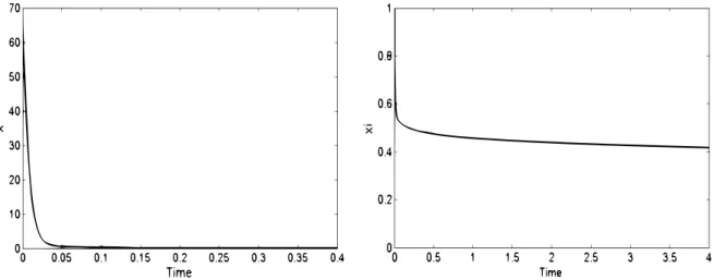
Example 5.1. The scalar system

RD^αx =−x can be expressed as _dt^dξ(t) =−^RD^1−αξ, or by integration,

ξ(t) =ξ(0)−

Z d dtI^1−αξ.

Using the NID-block of Matlab/Simulink, where the fractional integral is approximated in the Laplace domain by integer filters, this system is simulated in Fig.5.1, withα=0.9 and ξ(0) = 1. It is seen that x(0)takes high values near zero (in theory, lim_t→0⁺x(t) = +_∞ and limt→_∞x(t) =_{0) and}ξ is decreasing, since its integer derivative is−x.

Figure 5.1: Time evolution of functionsx(on the left) and ξ (on the right).

5.2 Caputo systems

To enlarge the application of our results, we show a way to associate a RL system to Caputo one. Consider the Caputo system

(CD^αx= f(x,t)

x(0) =x0∈ _Rⁿ, (5.1)

where x(t),f(x,t) ∈ _Rⁿ for all t > 0 and 0 < α ≤ 1. The solutions to this system areC[0,T] provided that, for instance, f is Lipschitz continuous in its first argument. Using [15, eq.

2.4.8],

CD^αx = ^RD^αx−x(0)t^−α, we obtain the following RL associated system

(RD^αx= f(x,t) +x(0)t^−α =: ˜f(x,t) x(₀) =x₀∈_Rⁿ_.

However, its initial condition is finite kx(0)k < _∞ and the solution is continuous at [_0,T] _{for every T} > 0. Hence, the RL system must have null initial condition, that is, lim_t→0I^1−αx(t) = 0, and then the forcing function x(0)t^−α yields nontrivial solutions. Con- sider as an example the scalar case f(x) =ax. Then, the associated RL system is given by

(_R

D^αx= ax+_Γ(^x(0)

1−α)t^−α lim_t→0I^1−αx(t) =0.

The solution to this equation would be given by [15, eq. 4.1.14]

x(t) = ^x(0) Γ(1−α)

Z _t

0

(t−τ)^α−1E_α,α(a(t−τ)^α)τ^−αdτ,

but note that the forcing function is not continuous at zero. Equaling to the known solution of the Caputo initial problem, we must have

1 Γ(₁−α)

Z _t

0

(t−τ)^α−1E_α,α(a(t−τ)^α)τ^−αdτ≡E_α(at^α),

which is an equality in Laplace domain, since L[t^α−1E_α,α(at^α)](s) = _sα¹_+a, L_Γ(^t−α

1−α)

(s) = s^α−1 andL[E_α(at^α)](s) = _s^s_α^α₊⁻¹_a.

Acknowledgements

The first author thanks to ‘CONICYTPCHA/National PhD scholarship program, 2018’. The second author thanks to CONICYT Chile for the support under Grant No FB0809 “Centro de Tecnología para la Minería”.

References

[1] A. Alikhanov, A priori estimates for solutions of boundary value problems for fractional-order equations, Differ. Uravn. 46(2010), 660–666. https://doi.org/10.1134/

S0012266110050058;MR2797545

[2] A. Alsaedi, B. Ahmad, M. Kirane, Maximum principle for certain generalized time and space fractional diffusion equations, Quart. Appl. Math. 73(2015), 163–175. https:

//doi.org/10.1090/S0033-569X-2015-01386-2;MR3322729

[3] I. Bachar, H. Mâagli, V. D. Radulescu˘ , Positive solutions for superlinear Riemann–

Liouville fractional boundary-value problems, Electron. J. Differential Equations 2017, No. 240, 1–16.MR3711193

[4] P. Clement, J. A. Nohel, Asymptotic behavior of solutions of nonlinear Volterra equa- tions with completely positive kernels, SIAM J. Math. Anal. 12(1981), 514–534. https:

//doi.org/10.1137/0512045;MR617711

[5] N. Cong, T. Doan, H. Tuan, Asymptotic stability of linear fractional systems with con- stant coefficients and small time dependent perturbations, Vietnam J. Math. 46(2018), No. 3, 665–680.https://doi.org/10.1007/s10013-018-0272-4;MR3820455

[6] N. Cong, T. Doan, S. Siegmund, H. Tuan, Linearized asymptotic stability for fractional differential equations, Electron. J. Qual. Theory Differ. Equ. 2016, No. 39, 1–13. https://

doi.org/10.14232/ejqtde.2016.1.39;MR3513975

[7] K. Diethelm, The analysis of fractional differential equations. An application-oriented ex- position using differential operators of Caputo type, Lecture Notes in Mathematics, Vol. 2004, Springer-Verlag, Berlin, 2010.https://doi.org/10.1007/978-3-642-14574-2; MR2680847

[8] M. A. Duarte-Mermoud, N. Aguila-Camacho, J. A. Gallegos, R. Castro-Linares, Using general quadratic Lyapunov functions to prove Lyapunov uniform stability for fractional order systems,Commun. Nonlinear Sci. Numer. Simul. 22(2014), No. 1, 650–659.

https://doi.org/10.1016/j.cnsns.2014.01.022;MR3282452

[9] J. A. Gallegos, N. Aguila-Camacho, M. A. Duarte-Mermoud, Smooth solutions to mixed-order fractional differential systems with applications to stability analysis,J. Inte- gral Equations Appl., accepted.

[10] J. A. Gallegos, M. A. Duarte-Mermoud, On the Lyapunov theory for fractional or- der systems, Appl. Math. Comput.287(2016), 161–170.https://doi.org/10.1016/j.amc.

2016.04.039;MR3506517

[11] J. A. Gallegos, M. A. Duarte-Mermoud, N. Aguila-Camacho, R. Castro-Linares, On fractional extensions of Barbalat Lemma, Syst. Control Lett. 84(2015), 7–12. https:

//doi.org/10.1016/j.sysconle.2015.07.004;MR3391078

[12] W. Glockle, T. Nonnenmacher, A fractional calculus approach of self-similar pro- tein dynamics, Biophys. J. 68(1995), 46–53. https://doi.org/10.1016/S0006-3495(95) 80157-8

[13] R. Hilfer, Applications of fractional calculus in physics, World Scientific, Singapore, 2000.

https://doi.org/10.1142/9789812817747MR1890104

[14] H. K. Khalil, Nonlinear systems, 2nd ed., Englewood Cliffs, NJ: Prentice Hall, 1996.

Zbl 1003.34002

[15] A. A. Kilbas, H. M. Srivastava, J. Juan Trujillo, Theory and applications of fractional differential equations, North-Holland Mathematics Studies, Vol. 204, Elsevier Science B.V., Amsterdam, 2006.https://doi.org/10.1016/S0304-0208(06)80001-0;MR2218073 [16] Y. Li, Y. Chen, I. Podlubny, Stability of fractional-order nonlinear dynamic systems:

Lyapunov direct method and generalized Mittag-Leffler stability, Comput. Math. Appl.

59(2010), 1810–1821.https://doi.org/10.1016/j.camwa.2009.08.019;MR2595955 [17] S. Liu, X. Wu, X. Zhou, W. Jiang, Asymptotical stability of Riemann–Liouville frac-

tional nonlinear systems,Nonlinear Dynam. 86(2016), 65–71. https://doi.org/10.1007/

s11071-016-2872-4;MR3545550

[18] K. Narendra, A. Annaswamy, Stable adaptive systems, Dover Publications: New York, USA, 2005.https://doi.org/10.1002/acs.4480040212

[19] D. Qian, C. Li, R. Agarwal, P. Wong, Stability analysis of fractional differential system with Riemann–Liouville derivative, Math. Comput. Modelling 52(2010), 862–874. https:

//doi.org/10.1016/j.mcm.2010.05.016;MR2661771

[20] J. Slotine, W. Li,Applied nonlinear control, Prentice-Hall, 1991.Zbl 0753.93036

[21] H. T. Tuan, A. Czornik, J. Nieto, M. Niezabitowski, Global attractivity for some classes of Riemann–Liouville fractional differential systems. https://arxiv.org/abs/

1709.00210v2.