Reduced linear fractional representation of nonlinear systems for stability analysis ?

Reduced linear fractional representation of nonlinear systems for stability analysis ?

P´eter Polcz^∗ Tam´as P´eni^∗∗ G´abor Szederk´enyi^∗,∗∗

∗Faculty of Information Technology and Bionics, P´azm´any P´eter Catholic University, Pr´ater u. 50/a, H-1083 Budapest, Hungary

(email: polcz.peter@itk.ppke.hu)

∗∗Systems and Control Laboratory, Institute for Computer Science and Control (MTA SZTAKI), Hungarian Academy of Sciences, Kende u.

13-17, H-1111 Budapest, Hungary

Abstract:Based on symbolic and numeric manipulations, a model simplification technique is proposed in this paper for the linear fractional representation (LFR) and for the differential algebraic representation introduced by Trofino and Dezuo (2013). This representation is needed for computational Lyapunov stability analysis of uncertain rational nonlinear systems. The structure of the parameterized rational Lyapunov function is generated from the linear fractional representation (LFR) of the system model. The developed method is briefly compared to the n-D order reduction technique known from the literature. The proposed model transformations does not affect the structure of Lyapunov function candidate, preserves the well-posedness of the LFR and guarantees that the resulting uncertainty block is at most the same dimensional as the initial one. The applicability of the proposed method is illustrated on two examples.

Keywords:Linear fractional representation, computational methods, stability analysis, Lyapunov functions, model simplification

1. INTRODUCTION

Finding or at least approximating the domain of attraction (DOA) of nonlinear dynamical systems is an important task in model analysis and controller design/evaluation, and numerous works have been devoted to this issue, see, e.g. Vannelli and Vidyasagar (1985); Rozgonyi et al.

(2010); Ohta et al. (1993); Giesl and Hafstein (2012).

In the last two decades, the theory of linear matrix in- equalities (LMI) and convex optimization alongside with nonlinear system modeling have made a considerable progress, which provide powerful and efficient tools to model and solve robust control, stability and filtering problems through LMI techniques. Ghaoui and Scorletti (1996) used quadratic Lyapunov functions (LF) and linear fractional transformation (LFT) to represent a rational nonlinear system and defined convex conditions for sta- bility analysis and state feedback design. Trofino et al.

(2013) considered uncertain rational LFs, moreover, affine annihilators and Finsler’s lemma was used to formulate parameter dependent LMI conditions for the stability of uncertain rational nonlinear systems. The obtained LMIs were solved within a bounded polytopic subset of the state space.

Although the above mentioned optimization based tech- niques are advantageous for DOA computation, they are

? The research was partially supported by the grant K115694 of the National Research, Development and Innovation Office - NKFIH.

The project has also been supported by the European Union, co- financed by the European Social Fund through the grant EFOP- 3.6.3-VEKOP-16-2017-00002. The research leading to the results presented in the paper was supported (also) by the J´anos Bolyai Research Scholarship of the Hungarian Academy of Sciences.

less attractive from a computational point of view. In general, they result in a high-dimensional optimization model, which is difficult to solve. In order to make these procedures numerically tractable, several dimension re- duction techniques have been developed. Trofino et al.

(2013) showed that omitting certain irrelevant nonlinear terms from the structure of the LF may result in a good estimate of the DOA with less computational effort. Polcz et al. (2017) used LFT and further automatic algebraic simplification steps to generate a reduced set of non- linear terms considered in the LF. Both techniques op- erate on the differential-algebraic system representation needed for DOA computation and introduced by Trofino et al. (2013). At the same time, LFT provides several dimension reduction possibilities, e.g. Marcos et al. (2005);

Hecker and Varga (2005, 2006); Hecker (2008) proposed symbolic preprocessing and matrix conversion techniques for low-order LFT modeling, such as Horner factoriza- tion, continued-fraction form, enhanced tree decomposi- tion, Morton’s method, enhanced variable splitting factor- ization, etc. These new symbolic manipulation techniques are implemented in the sym2lfr function of Enhanced LFR-toolbox for Matlab (Hecker et al. (2004)), henceforth is referred to as theLFR-toolbox.

After the LFT, the obtained linear fraction representa- tion (LFR) can be considered as a generalized state-space model, on which further numerical order reduction tech- niques can be applied. Lambrechts et al. (1993) proposed a standard 1-D order reduction (1-DOR) for the LFR, which removes the unobservable/uncontrollable eigenval- ues from each subsystem of the LFR corresponding to each

uncertainty block. Based on a Kalman like decomposition, D’Andrea and Khatri (1997) proposed the n-D order re- duction (n-DOR), which is proved to be less conservative than 1-DOR, since it considers all uncertainty blocks at the same time. The n-DOR is implemented in the LFR-toolbox function minlfr. According to Magni (2006), numerical order reduction techniques of the LFR-toolbox consider strong input/output equivalence of the LFR models. Based on this equivalence relation of LFRs introduced by Doyle et al. (1996), Magni (2006) defined the notion ofminimal- ity andrelative-minimality of an LFR model. An LFR is said to beminimal if there is no equivalent representation with a smaller uncertainty block (∆). Furthermore, an LFR is said to berelative-minimal if there is no similarity transformation, such that some states can be eliminated without modifying the input/output characteristics of the LFR. It is shown by D’Andrea and Khatri (1997) that the n-DOR leads to a relative-minimal representation.

In this paper, we consider uncertain rational nonlinear systems in the lower LFR (Lambrechts et al. (1993)), that is generated using the systematic symbolic manipulation techniques contained in the functionsym2lfrof the LFR- toolbox. In general, the obtained model is reducible, there- fore, we have the possibility to apply the available order reduction techniques. The structure of the LF candidate is given by a set of rational uncertain terms, which are generated from the LFR by using symbolic computations.

Nevertheless, it is stated by Varga and Looye (1999), that

“the interlaced symbolic and numeric manipulations are hazardous since they involve many tolerance dependent rank decisions”. Additionally, due to the “fraction of in- tegers” symbolic representation of floating point numbers, numerical reduction may lead to very complex symbolic expressions in the LF. On the other hand, after a numerical reduction, the obtained LFR may generate a reduced set of rational functions, hence eliminating certain (maybe important) rational terms from the structure of the LF.

As a possible resolution, we propose a symbolic model sim- plification method, which, compared to n-DOR, generates an LFR containing a possibly higher dimensional uncer- tainty block, but having advantageous properties for DOA estimate computation. And, importantly, it preserves the structure of the LF candidate.

1.1 The studied uncertain system class

We consider nonlinear systems in the quasi linear param- eter varying (quasi-LPV) form

˙

x(t) =A(x(t), δ)x(t), x(t)∈Rⁿ, x₀∈ X, δ∈ D (1) where x(t) ∈ Rⁿ is the state vector, x(0) = x0 is the initial condition, and δ ∈ R^d is a vector of constant uncertain parameters.X ⊂Rⁿ and D ⊂R^d are bounded polytopes given a priori. Polytope X is the set of initial states considered in the stability analysis. We assume that A(x, δ) is a matrix of well-defined scalar uncertainrational functions a_ij(x, δ), i, j = 1, n. Secondly, we assume that the origin x^∗ = 0n ∈ X is an asymptotically stable equilibrium point of (1) for all δ ∈ D. From now on, the time argument ofxwill be suppressed. We denote the bounded s-dimensional polytopeX ×D ⊂R^s by Ω, where s:=n+d. We use the vector valued variableω= (^x_δ)∈Ω as a shorthand for the arguments of an arbitrary function f depending both on x and δ, namely f(ω) := f(x, δ).

Finally, let 0n ∈Rⁿ, andIn∈R^n×ndenote the zero vector and the identity matrix, respectively.

1.2 Model representation and Lyapunov functions Similarly to Trofino et al. (2013), we propose to start from the following differential algebraic representation of (1) needed for stability analysis:

˙

x=A(ω)x=Ax+Bπ(ω), π(ω)∈R^p, (2a) where A ∈ R^n×n, B ∈ R^n×p are constant matrices, and π(ω) ∈ R^p is a vector of well-defined uncertain rational nonlinear functions of ω. Furthermore, we consider the algebraic constraint:

0p=G(ω)x+F(ω)π(ω), ∀ω∈Ω, (2b) which represents the algebraic coupling between the state variables and the nonlinear uncertain terms of the system equationA(ω)xcollected in vectorπ(ω).G(ω)∈R^p×nand F(ω)∈R^p×p are matrices ofaffine functions ofω. Matrix F(ω) is assumed to benon-singular for allω∈Ω.

With reference to Trofino et al. (2013), a suitable LF is searched in the form

V(ω) =π^T_b(ω)P π_b(ω), π_b(ω) = _π(ω)^x

∈R^m:=n+p (3) where P ∈ R^m×m is a (not necessarily positive definite) symmetric matrix. The combined vectorπb(x, δ) contains the rational terms to be considered in the LF. The neces- sary Lyapunov conditions for local stability, namely

vl(kxk)≤V(ω)≤vu(kxk) ∀ω∈Ω, (4a) V˙(ω) := ∂V(ω)/∂xA(ω)x≤ −v_d(kxk) ∀ω∈Ω, (4b) are ensured using sufficient LMI conditions, where vl(·), v_u(·) andv_d(·) are continuous strictly increasing functions, being zero inx= 0. Trofino et al. (2013) introduced further LMI conditions to ensure that the unitary level set of the LF is entirely inside of X for all δ ∈ D. Additionally, a linear objective function is proposed and meant to be minimized in order to enlarge the unitary level set as much as possible. After the LF computation, the maximal stability domain inside X can be characterized by the following two regions

I={x∈ X | ∀δ∈ D:V(x, δ)≤1},

U={x∈ X | ∃δ∈ D:V(x, δ)≤1}, I⊆U. (5) Due to the Lyapunov conditions it is ensured that any trajectory with an initial condition fromIwill not leaveU.

The proposed LMI optimization problem of Trofino et al.

(2013) in equation (91) can be efficiently solved by the available numerical tools, although, the sizes of the ob- tained LMIs explode combinatorially as the number of coordinates of π(ω) ∈ R^p increase. Therefore, the di- mension reduction of the optimization model needs to be addressed in order that the method be adoptable on complex and/or higher dimensional systems. At the same time, there is a trade-off between the model’s dimension and the conservatism of the obtained estimate, since any new term inπ(ω) may result in a better LF with a larger stability region estimateI(see e.g. Section 5.2).

In order to reduce the dimension ofπ(ω) appearing in (2), Polcz et al. (2017) proposed systematic algebraic simpli- fication steps, which resulted in a significant dimension reduction of the optimization problem. However, the pro- posed algebraic manipulations do not preserve the non- singularity of matrixF(x), and it is generally not assured

that F(x) remains a square matrix. Nevertheless, Theo- rem 4.1 of Trofino et al. (2013), related to local stability, requires the non-singularity of the square matrix F(ω).

Furthermore, in certain cases, the proposed simplification steps may result in an even higher dimensional model as the initial one.

2. LINEAR FRACTIONAL TRANSFORMATION LFT plays an important role in modeling uncertain ratio- nal systems, and it is often used in literature, as presented by Ghaoui and Scorletti (1996). Using the LFT any quasi- LPV system of the form (1) can be represented as a linear time invariant (LTI) system:

˙

x=Ax+Bπ, A∈R^n×n, B∈R^n×p, (6a) y=Cx+Dπ, C∈R^p×n, D∈R^p×p, (6b) with a nonlinear input characterized by the operator ∆(ω):

π=π(ω) = ∆(ω)y, ∆ :R^n+d→R^p×p. (6c) In representation (6), A, B, C, D are constant matrices, x∈Rⁿ,π, y∈R^pare the state, input, and output vectors, respectively. Henceforth, (6) will be shortly denoted by Fp(A, B, C, D; ∆), which is a lower LFR of matrixA(ω).

Subscript pemphasizes the dimension of the uncertainty block ∆(ω) of the LFR.

Multiplying (6b) by ∆(ω) from the left, and using (6c), we obtain an algebraic relation (2b) between xandπ(ω),

whereG(ω) :=−∆(ω)C∈R^p×n, (7a) F(ω) :=Ip−∆(ω)D∈R^p×p. (7b) This LFR is well-posed (i.e. well-defined) since, by assump- tion,F(ω) is non-singular for allω∈Ω. Consequently, for each well-posed LFR, an explicit formula can be given for the set of rational functions considered in the LF (3):

π(ω) =−F(ω)⁻¹G(ω)x∈R^p. (7c) Although, the numerical n-DOR technique preserves the value of A(ω) =A−BF(ω)⁻¹G(ω), it may also remove certain rational terms from the generated vector π(ω) of the initial LFR. On the other hand, the symbolic calculation of F(ω)⁻¹ for the numerically reduced LFR may be difficult.

In Section 3, we introduce a symbolic preprocessing step, a decomposition of vector πb(ω), then, in Section 4, we propose a model simplification method for representation (2), which decreases the dimension of π(ω) (if possible), such that the structure of the initial LF (3) remains the same.

3. CANONICAL DECOMPOSITION OF A VECTOR OF RATIONAL FUNCTIONS

In this section, the vector valued variables z(ω), ˇz(ω),∈ R^m and z0(ω)∈R^K will be denoted as bold symbols, in order to emphasize the distinction between them and their (scalar valued) coordinate valueszi(ω), ˇzi(ω), andz0,j(ω), wherei= 1, mandj= 1, K.

Letz(ω)∈R^m, be a vector ofrational functions, namely z(ω) =z₁(ω)

...

z_m(ω)

, zi(ω) =u_i(ω)

vi(ω), i= 1, m, (8)

Procedure 1.Decomposition ofz(ω).

1: procedureDecompose(z(ω) ∈ R^m)

2: v(ω;κ)← hκ,z(ω)i, whereκ∈R^1×m,ω∈R^s

3: ˇv(ω;κ),q(ω)←NumDen(v(ω;κ))

4: cj(κ),z0,j(ω)←Coeffs(ˇv(ω;κ), ω), wherej= 1, K

5: z0(ω)←(z_0,1(ω)... z_0,K(ω))^T

6: Θ←EquationsToMatrix(c1(κ), ..., c2(κ), κ)

7: returnΘ,z0(ω),q(ω)

8: end procedure

where ui(ω) and vi(ω) are multivariate polynomials of ω1, ..., ωs ∈ R (i.e. in short ω ∈ R^s) and vi(ω) 6= 0 for allω∈Ω. We aim to find the following decomposition

z(ω) = Θz₀(ω)q(ω)⁻¹, (9) where Θ∈R^m×K is a constantcoefficient matrix ofz(ω), q(ω) is amonic polynomial of ω (with leading coefficient 1), andz0(ω)∈R^K is a vector, in which the coordinates z0,j(ω) are distinct monic monomials,j= 1, K.

In order to perform this decomposition, first we determine the smallest degree common monic denominator q(ω) of rational functions z₁(ω), ..., z_m(ω). We introduce vector ˇ

z(ω) := z(ω)q(ω), in which the coordinates functions are polynomials, and let z₀(ω) contain every distinct monomial term, which appears in each coordinate of ˇz(ω).

Then, for each ˇzi there exist real valuesϑij∈Rsuch that ˇ

zi(ω) =

P

j=1ϑijz0,j(ω), i= 1, m. (10) Finally, ˇz(ω) can be written as:

ˇ

z(ω) = Θz₀(ω), Θ :=ϑ₁₁ ... ϑ_1K ... ...

ϑm1... ϑmK

∈R^m×K, (11) which gives the decomposition (9) of vectorz(ω).

The proposed decomposition described in Procedure 1 can be efficiently produced using Matlab’s Symbolic Math Toolbox (SMT). In order to compute q(ω), we introduce m number of auxiliary symbolic (indetermi- nate) scalar variablesκ1, ..., κm, collected in a row vector κ= (κ1 ... κm)∈R^1×m. The operations of Procedure 1 are explained below in the following list, where the num- bers correspond to the line numbers of Procedure 1:

2. Evaluate the dot product ofhκ,z(ω)i=:v(ω;κ). Both κ and ω are vectors of symbolic variables. z(ω) ∈ R^m is a vector of ω-dependent symbolic rational expressions. The resulting scalar valued objectv(ω, κ) is a rational expression of indeterminatesω andκ.

3. Reduce v(ω;κ) into an irreducible fractional form, then determine the resulting numerator ˇv(ω;κ) :=

hκ,z(ω)iˇ and denominator q(ω). These operations can be automated using the SMT functionnumden.

4. Collect and extract the multipliers of the common monomial terms (z0,j(ω)) of the numerator ˇv(ω;κ) with respect to variables ω1, ..., ωs:

ˇ

v(ω;κ) =Pm

i=1κizˇi(ω) =PK

j=1cj(κ)z0,j(ω), (12) where the multipliers cj(κ) = Pm

i=1κiϑij are linear functions of indeterminates κ₁, ..., κ_m, furthermore, z0,j(ω) is the corresponding monomial term. These pairs can be extracted using SMT functioncoeffs.

5. Let the coordinates of z0(ω) be the resulting mono- mialsz0,j(ω) in the same order as it was returned by SMT functions coeffs.

6. Using SMT functionequationsToMatrix, determine the coefficients ϑ1j, ..., ϑmj for each multiplier cj(κ) returned by SMT functions coeffs, then construct the coefficient matrix Θ∈R^m×Kas presented in (11).

7. This procedure will return matrix Θ, vector z0(ω) with distinct monic monomial coordinates functions and the denominator q(ω), which together will give the desired decomposition ofz(ω).

Note that for a fixed monomial order, this decomposition is unique.

4. MODEL SIMPLIFICATION

In this section, we propose a linear (similarity) transfor- mation of the LFR, which imply that some variables in vectors π andy and the corresponding equations in (6b) can be eliminated from the LFR without modifying both the value of the uncertain matrix A(ω), and the set of uncertain rational terms of the LF candidate.

We consider a system in representation (6) with the vector π_b(ω) = _π(ω)^x

. As presented in (9), we produce the decomposition ofπb(ω) as follows:

πb(ω) = Θπ0(ω)q(ω)⁻¹∈R^m=n+p. (13) If Θ∈R^m×K is full row-rank, our method cannot reduce the model’s dimension. Let the rank of Θ be n+k < m, than Θ can be written in the following block-matrix form:

Θ =



 Θx

Θπ1

Θ_π2



∈R^m×K, Θx∈R^n×K, Θπ₁ ∈R^k×K Θπ₂ ∈R^(p−k)×K. (14) Proposition 1. Matrix Θ_x∈R^n×K is full row-rank.

Proof. Suppose that Θ_x=_ϑ1

...

ϑ_n

is rank deficient. Then, there exists an indexj and real valuesβ_i, such that

ϑj=Pn

i=1,i6=jβiϑi, 1≤j≤n. (15) Considering the dot product of both sides of (15) with π0(ω)q(ω)⁻¹ we obtain thatxj =Pn

i=1,i6=jβixi, which is a contradiction, since generally, there is no linear depen- dence between the state variables. Consequently, Θxmust be a full row-rank matrix.

After an appropriate permutation of coordinates in vector π(ω) of model (6), we may assume, without the loss of generality, that Θπ₁ is full row-rank. Consequently, there exist matrices Γ1∈R^(p−k)×n and Γ2∈R^(p−k)×k such that

Θ_π2 = Γ₁Θ_x+ Γ₂Θ_π1. (16) Namely, the rows of Θπ₂ can be expressed as the linear combination of the rows in matrices Θ_xand Θ_π1.

Let us introduce the following decompositions of (6):

˙

x=Ax+B1π1+B2π2, (17a) y₁=C₁x+D₁₁π₁+D₁₂π₂, (17b) y2=C2x+D21π1+D22π2, (17c)

π1= ∆1(ω)y1, (17d) π₂= ∆₂(ω)y₂, (17e) wherey1∈R^k andπ1∈R^k,k < pare the output and the nonlinear input, respectively.

Proposition 2. If we introduce the transformed matrices Ab:=A+B2Γ1, Bb:=B1+B2Γ2,

Cb:=C1+D12Γ1, Db:=D11+D12Γ2, (18)

representation Fk(A,b B,b C,b D; ∆b ₁), with π₁ and y₁ is a dimensionally reduced equivalent of (6). Furthermore, Fk(A,b B,b C,b D; ∆b 1) is well-posed if (6) is well-posed.

Proof. Due to (16), there exists a matrixS∈R^m×m, S=





I_n 0 0 0 I_k 0

−Γ1 −Γ2Ip−k



, s.t.S·Θ =



 Θ_x Θ_π1 0



. (19) Multiplying both sides of the second equation of (19) with π0(ω)q(ω)⁻¹, we obtain a key identity forπ2

S·



 x π₁ π2



=



 x π₁ 0



 ⇒ π2= Γ1x+ Γ2π1. (20) Considering (20), the state and output equations (17a,17b) of representation (17) are rewritten as

˙

x= (A+B2Γ1)x+ (B1+B2Γ2)π1, (21a) y₁= (C₁+D₁₂Γ₁)x+ (D₁₁+D₁₂Γ₂)π₁, (21b)

withπ1= ∆1(ω)y1. (21c)

The output equation (17c) of y2 and (17e) can be sup- pressed, since the system dynamics (21a) does not depend onπ₂ nor on y₂. Representation (21) describes the same dynamics as the original (decomposed) model (17).

Using the inverse ofS, vectorπ_b(ω) can be given as follows:

πb(ω) =S⁻¹



 x π₁ 0



, withS⁻¹=





I_n 0 0 0 I_k 0 Γ1Γ2 Ip−k



. (22) On the other hand, considering the block-matrix decom- position of matricesG(ω) andF(ω) of (7), we have that

kl p−kl

G1(ω) n

F11(ω) k

F12(ω) p−k G2(ω) F21(ω) F22(ω)

! x π₁(ω) π₂(ω)

!

= 0. (23) Using (22), and considering only the upper part (first k rows) of identity (23), we reach to the following identity:

G₁(ω) +F₁₂(ω)Γ₁ x+

F₁₁(ω) +F₁₂(ω)Γ₂

π₁(ω) = 0.

Note that (F₁₁(ω) F₁₂(ω)) and _Γ^Ik

2

are full row-, and column-rank matrices, respectively, thus their product F(ω) :=b F11(ω) +F12(ω)Γ2 is non-singular, hence invert- ible, and π₁(ω) =−F(ω)b ⁻¹G(ω)xb with G(ω) =b G₁(ω) + F12(ω)Γ1, which completes the proof.

Proposition 3.(Structure invariance of the LF). Let πb(ω) =

_x

π₁(ω) π2(ω)

, and bπb(ω) = x

π1(ω)

. (24) Then, for every matrixP ∈R^m×m there exists a matrix Pb∈R(n+k)×(n+k), such that

V(ω) =π^T_b(ω)P πb(ω) =bπ_b^T(ω)Pbπbb(ω),∀ω∈R^n+d. (25) Proof. We introduce the block-matrix decomposition of matrixP of the LFV(ω) in (25):

P =

P₁₁ P₁₂ P21 P22

, whereP₁₁∈R(n+k)×(n+k). (26) Considering (22), the LF (25) can be altered as follows:

π_b^TP πb = πb^T_b 0 S^−T

P11 P12

P₂₁ P₂₂

S⁻¹

πbb

0

(27)

=πb^T_b P11+Γ^TP21+P12Γ+Γ^TP22Γ

bπb=:πb^T_bPbπbb, where Γ := (Γ1 Γ2). Consequently, we obtained that P withπb andPb withbπb satisfies (25) for everyω∈R^s.

−0.5 0 0.5

−2

−1 0 1

X

state variable (x)

˙x=A(x)x

−0.50 0 0.5 0.5

1

X state variable (x)

Lyapunovf.V(x)

Fig. 1. Plot of ˙xversusxfor 1D system (28) (left).x^∗= 0 is a (locally) stable equilibrium point, since the graph crosses axis x with a negative slope. The obtained rational LF for (28) is illustrated in the right figure.

The red line segment highlights polytopeX.

To conclude, the proposed linear transformation (18) re- sults in a simplified LFR model (i.e. with a smaller uncertainty bock ∆1). Furthermore, the obtained LFR Fk(A,b B,b C,b D; ∆b 1) generates the same rational terms to be considered in the LF as the initial LFR model.

5. ILLUSTRATIVE NUMERICAL EXAMPLES In this section, we illustrate the applicability of the ap- proach presented above through different numerical ex- amples. The results presented in this section were com- puted in the Matlab environment. For symbolic computa- tions, we applied Matlab’s built-in Symbolic Math Tool- box based on Mupad. To model and solve semidefinite optimization (SDP) problems, we used YALMIP, L¨ofberg (2004), with Mosek solver, MOSEK ApS (2015). We used LFT software tools provided by the LFR-toolbox.

5.1 One dimensional benchmark system

In order to transparently illustrate the difference between the n-DOR, the symbolic manipulations of Polcz et al.

(2017), and the proposed model reduction, we consider a very simple artificial one dimensional benchmark system:

˙

x=A(x)x, where A(x) = _x+1¹ +_x3+x2¹_+x+1−4. (28) If the domain of operation is constrained to x(t) ∈ (−1,∞), this system is well-defined and it has a locally stable equilibrium point at x^∗ = 0, for which the DOA can be determined precisely considering the graph of ˙x= A(x)xversus the state variablex(Fig. 1). The reason we still use this 1D model is to demonstrate the operations of the proposed model reduction method, and to show its possible advantages compared to the two other mentioned techniques know from the literature. The set of possible initial conditions considered in the stability analysis is chosen to be X = [−0.5,0.5].

Applying LFR-toolbox function sym2lfrtoA(x), an ini- tial 4-dimensional LFR model is obtained:

Ae=−2, Be= (^{−1 0 0−1}), (29a) Ce=

₁

1 1 1

, De =

−1 1 0 0

−1 0 1 0

−1 0 0 0 0 0 0−1

, ∆(x) =e xI₄. The generated set of rational terms to appear in the LF is

eπ(x) = _x4 1+x3

1+x2 1 x3

1+x2 1+x1 +1

x2 1 x2

1+1 x2

1 x3

1+x2 1+x1 +1

x2 1 x1 +1

T

(29b) The numerical n-DOR technique results in a 3-dimensional LFR (A.1a), for which the obtained rational terms are

presented in (A.1b). The symbolic simplification steps for model (29) proposed by Polcz et al. (2017) generates a 5-dimensional model (A.2) with a set of rational terms, in which both the denominators and the monomial nu- merators are monic. Using the proposed model simpli- fication technique presented in Section 4, we obtain a 3-dimensional LFR (A.3), for which the corresponding rational functions inπ(ω) are relatively simple compared to the model (A.1a) generated by the n-DOR.

5.2 An uncertain mass-action kinetic (MAK) system We consider the minimal MAK system presented by Wil- helm (2009) with a modified parameter configuration and with an uncertain reaction rate coefficientδ:

˙¯

x₁=v₁−δ¯x₁x¯²₂,

˙¯

x2=δ¯x1x¯²₂−k2x¯2, where δ∈ D= [0.8,1.2], k2= 2, v1= 4. (30) This system with the given parameter values has a locally asymptotically stable equilibrium point at ¯x^∗(δ) = (¹δ 2)^T with an unbounded DOA. The task is to generate a model (2) and then give a (bounded) estimate for the DOA by solving the optimization problem given in (91) of Trofino et al. (2013).

Introducing the centered state vector x := ¯x−x¯^∗ and considering the numerical values of coefficientsv₁andk₂, we obtain a system ˙x=A(x, δ)x, where:

A(ω) =

−δ(x2+ 2)² −x2−4 δ(x₂+ 2)² x₂+ 2

. (31)

Applying the LFR-toolbox functionsym2lfrtoA(ω), we obtain a 8-dimensional LFR model. The numerical n-DOR results in a 3-dimensional LFR. The corresponding set of rational terms is denoted by π⁰(ω). The proposed LFR transformation produces a 4-dimensional model withπ(ω).

The values of both vectors π⁰(ω) and π(ω) are given in (A.4). For this system, the algebraic simplifications of Polcz et al. (2017) generates a 4-dimensional model.

Consider the following tworectangular polytopes

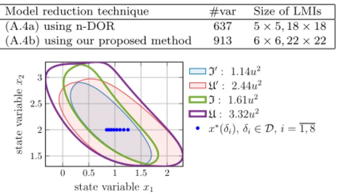
X1= [−1.4,1.4]×[−0.7,1.3],X2= [−1.9,1.9]×[−0.7,1.5]. (32) We solved the DOA computation problem (91) of Trofino et al. (2013) for both polytopes and both (simplified) models (A.4). For model (A.4a) with polytope X2, the problem is infeasible. The area of the estimated stability region in the different cases is given in Table 1.

Though the optimization is adopted on the centered sys- tem, the obtained LFV(x, δ) is transformed back into the original coordinate system ¯V(¯x, δ) =V(¯x−x¯^∗(δ), δ). Then the two regionsI⊂Uare computed similarly as presented in (5). The obtained areas are illustrated in Figure 2.

6. CONCLUSIONS

In this paper, we presented a model simplification tech- nique for the LFR based on symbolic and numeric manipu- lations. Using the obtained LFR with a reduced number of input-output pairs (πi, yi), a specific system representation is generated, which is used for the DOA estimate computa- tion for rational uncertain nonlinear systems, as proposed by Trofino et al. (2013). The structure of the Lyapunov function candidate is given by a set of rational uncertain terms, which are generated from the dimensionally reduced LFR. Compared to n-DOR, our proposed technique results

Table 1. Area of the estimated stability region us- ing different polytopes and different sets of rational functions considered in the LF. The two values in the 3rd column is the area of the inner and outer regions,

respectively, introduced in (5).

Model reduction technique X· Area (A.4a) using n-DOR X1 1.14,2.44u² (A.4a) using n-DOR X₂ infeasible (A.4b) using our proposed method X₁ 1.57,3.17u² (A.4b) using our proposed method X2 1.61,3.32u²

Table 2. Number of free decision variables of the optimization problem are given in the 2nd column for each model. The 3rd column gives the dimensions of the LMIs corresponding to the Lyapunov conditions (4).

Model reduction technique #var Size of LMIs (A.4a) using n-DOR 637 5×5,18×18 (A.4b) using our proposed method 913 6×6,22×22

0 0.5 1 1.5 2

1.5 2 2.5 3

state variablex₁

statevariablex2 I⁰: 1.14u²

U⁰: 2.44u² I: 1.61u² U: 3.32u²

x^∗(δ_i),δ_i∈ D,i= 1,8

Fig. 2. Computed stability regions for the minimal MAK system using both sets of rational function (A.4).

in a possibly higher dimensional model (i.e. with larger

∆ block), but all distinct rational terms of the initial LFR representation are preserved. The illustrative exam- ples show that the method is indeed suitable for DOA estimation.

REFERENCES

D’Andrea, R. and Khatri, S. (1997). Kalman decomposition of linear fractional transformation representations and minimal- ity. In Proceedings of the 1997 American Control Confer- ence (Cat. No.97CH36041), volume 6, 3557–3561 vol.6. doi:

10.1109/ACC.1997.609484.

Doyle, J.C., Paganini, F., D’Andrea, R., and Khatri, S. (1996). Ap- proximate behaviors. InDecision and Control, 1996., Proceedings of the 35th IEEE Conference on, volume 1, 688–693 vol.1. doi:

10.1109/CDC.1996.574430.

Ghaoui, L.E. and Scorletti, G. (1996). Control of rational systems us- ing linear-fractional representations and linear matrix inequalities.

Automatica, 32(9), 1273 – 1284. doi:10.1016/0005-1098(96)00071-4. Giesl, P. and Hafstein, S. (2012). Construction of Lyapunov functions for nonlinear planar systems by linear programming. Journal of Mathematical Analysis and Applications, 388, 463–479.

Hecker, S., Varga, A., and Magni, J.F. (2004). Enhanced LFR- toolbox for MATLAB. 25–29.

Hecker, S. (2008). Improved mu-analysis results by using low-order uncertainty modeling techniques. Journal of guidance, control, and dynamics, 31(4), 962–969.

Hecker, S. and Varga, A. (2005). Symbolic techniques for low order lft-modelling.

Hecker, S. and Varga, A. (2006). Symbolic manipulation tech- niques for low order lft-based parametric uncertainty mod- elling. International Journal of Control, 79(11), 1485–1494. doi:

10.1080/00207170600725644.

Lambrechts, P., Terlouw, J., Bennani, S., and Steinbuch, M. (1993).

Parametric uncertainty modeling using LFTs. 267–272.

L¨ofberg, J. (2004). Yalmip : A toolbox for modeling and optimization in MATLAB. InProceedings of the CACSD Conference. Taipei,

Taiwan. URLhttp://users.isy.liu.se/johanl/yalmip.

Magni, J.F. (2006). User Manual of the Linear Fractional Repre- sentation Toolbox: Version 2.0.

Marcos, A., Bates, D.G., and Postlethwaite, I. (2005). A multivariate polynomial matrix order-reduction algorithm for linear fractional transformation modelling.IFAC Proceedings Volumes, 38(1), 327 – 332. doi:http://dx.doi.org/10.3182/20050703-6-CZ-1902.00999.

16th IFAC World Congress.

MOSEK ApS (2015). The MOSEK optimization toolbox for MATLAB manual. Version 7.1 (Revision 28). URL http://docs.mosek.com.

Ohta, Y., Imanishi, H., Gong, L., and Haneda, H. (1993). Computer generated Lyapunov functions for a class of nonlinear systems.

IEEE Transactions on Circuits and Systems, 40, 343–354.

Polcz, P., P´eni, T., and Szederk´enyi, G. (2017). Improved algorithm for computing the domain of attraction of ratio- nal nonlinear systems. European Journal of Control. doi:

10.1016/j.ejcon.2017.10.003.

Rozgonyi, S., Hangos, K.M., and Szederk´enyi, G. (2010). Determin- ing the domain of attraction of hybrid non-linear systems using maximal Lyapunov functions.Kybernetika, 46, 19–37.

Trofino, A., Dezuo, T.J.M., Trofino, A., and Dezuo, T. (2013).

LMI stability conditions for uncertain rational nonlinear systems.

International Journal of Robust and Nonlinear Control, 24(18), 3124–3169. doi:10.1002/rnc.3047. Cited By 14.

Vannelli, A. and Vidyasagar, M. (1985). Maximal Lyapunov func- tions and domains of attraction for autonomous nonlinear sys- tems.Automatica, 21, 69–80.

Varga, A. and Looye, G. (1999). Symbolic and numerical software tools for lft-based low order uncertainty modeling. InComputer Aided Control System Design, 1999. Proceedings of the 1999 IEEE International Symposium on, 1–6. IEEE.

Wilhelm, T. (2009). The smallest chemical reaction system with bistability. BMC Systems Biology, 3(1), 90. doi:10.1186/1752- 0509-3-90. URL10.1186/1752-0509-3-90.

Appendix A. NUMERICAL VALUES

Matrices of the LFR and vectorπ(x) after using n-DOR on the initial LFR obtained for the benchmark 1D system:

A⁰=−2, B⁰= (0 0 1.4142), (A.1a)

C⁰=

−0.8165

−1.1547

−1.4142

, D⁰=

−0 −0.3536−0.5774 1.4142 0 −0.8165

−0 0.6124 −1

, ∆⁰=xI3. π⁰(x) =

_2.5e31x2(2.0e31x−4.1e31)

−1.4e32x²(1.0e31x+1.0e31)

−1.4x²(1.2e63x²+6.2e62x+1.2e63)

· 1

q(x), (A.1b) q(x) = 1.2e63x³+ 1.2e63x²+ 1.2e63x+ 1.2e63.

Simplified modeling as presented in Polcz et al. (2017):

B˘= (^{−1 0−1−1−1}), F˘(x) =

_{x+1−x x+1 0 x+1}

x 1 0 0 x

x 0 x+1 0 x

0 0 0 x+1 0

,

˘ π(x) =

x⁴

˘ q(x)

x² x²+ 1

x²

˘ q(x)

x² x+ 1

x³

˘ q(x)

, (A.2)

˘

q(x) =x³+x²+x+ 1.

LFR model and vectorπ(ω) after the proposed model simplification:

A=−2, B= (^{−2 1−1}), C=

₁

1 1

, D=

−1 1 0

−1 0 1

−1 0 0

, ∆(x) =xI3, π(x) =

_x4+x³+x² x³+x²+x+ 1

x² x²+ 1

x² x³+x²+x+ 1

(A.3) The set of rational functions considered in the LF for the uncertain MAK system generated by n-DOR (π⁰) and by the proposed model simplification technique (π):

π⁰(ω) =





−δx1

√ 2

1122⁻¹²·(δx1x2−8x²₂−8δx1x²₂) 66⁻¹2·(2x²₂+ 8δx1x2+ 2δx1x²₂)



 (A.4a)

π(ω) =

δx₁ δx1x²₂ 4 +δx₁x₂

2 δx₁x₂

2 x²₂ ^T

(A.4b)