Existence and Ulam type stability for nonlinear Riemann–Liouville fractional differential equations

Existence and Ulam type stability for nonlinear Riemann–Liouville fractional differential equations

with constant delay

Dedicated to Professor Jeffrey R. L. Webb on the occasion of his 75th birthday

Ravi Agarwal

, Snezhana Hristova

and Donal O’Regan

1Department of Mathematics, Texas A&M University-Kingsville, Kingsville, TX 78363, USA

2Distinguished University Professor of Mathematics, Florida Institute of Technology, Melbourne, FL 32901, USA

3Department of Applied Mathematics and Modeling, University of Plovdiv Paisii Hilendarski, Plovdiv, Bulgaria

4School of Mathematics, Statistics and Applied Mathematics, National University of Ireland, Galway, Ireland

Received 16 March 2020, appeared 21 December 2020 Communicated by Paul Eloe

Abstract. A nonlinear Riemann–Liouville fractional differential equation with constant delay is studied. Initially, some existence results are proved. Three Ulam type stability concepts are defined and studied. Several sufficient conditions are obtained. Some of the obtained results are illustrated on fractional biological models.

Keywords: Riemann–Liouville fractional derivative, constant delay, initial value prob- lem, existence, Ulam type stability.

2020 Mathematics Subject Classification: 34A08, 34K37, 34K20.

1 Introduction

Ulam type stability concept is quite significant in realistic problems in many applications in numerical analysis, optimization, biology and economics etc. This type of stability guaran- tees that there is a close exact solution. Recently, several authors extended and discussed Ulam type stability to fractional differential equations. The Ulam type stability is well stud- ied recently for Caputo fractional differential equations. For example, about Caputo frac- tional differential equations we refer [8,12], for Caputo fractional differential equations with impulses [14], about Caputo fractional differential equations with delays see, for example, [2,13], for ψ-Hilfer fractional derivative and a constant delay [11]. Note that in the case of

BCorresponding author. Email: agarwal@tamuk.edu

the Riemann–Louisville (RL) fractional derivative only the case without any delays is studied (see, for example, [3,7,13,16]).

In addition, many real world processes and phenomena are characterized by the influence of past values of the state variable on the recent one and this leads to the inclusion of delays in the models. The analysis of RL delay fractional differential equations is rather complex (ana- lytical solution computation, controllability analysis, etc.) and a very small class of equations could be solved in explicit form. It requires theoretical proofs of methods guarantee existence of enough close function to the unknown solution. One of these types of method is Ulam type stability. According to our knowledge this type of stability is not studied for nonlinear RL fractional differential equations with delays.

The main goal of the paper is to study scalar nonlinear RL fractional differential equations with a constant delay, to obtain some sufficient conditions for uniqueness and existence and to study Ulam type stability. The present paper is organized as follows. In Section 2, some notations and results about fractional calculus are given. In Section 3, an existence result, based on the Banach contraction principle, for the studied problem is presented. In Section 4, we prove three types of Ulam–Hyers stability results for the given RL fractional differential equation with a constant delay. Finally, in the last section, we illustrate the application of some of th obtained results on two fractional biological models: fractional generalization of Lasota–

Wa ˙zewska model and fractional generalization of the logistic equation with a biological delay depending on the mechanistic details of the model.

2 Preliminary notes on fractional derivatives and equations

In this section, we introduce notations, definitions, and preliminary facts which are used throughout the paper. LetT: 0<T< _{∞, ¯}J = [0,T], J = (0,T],τ>0 be given (the delay).

There exists a natural number N such that Nτ < T ≤ (N+1)τ holds, i.e. J =

∪^N_k=⁻₀¹(kτ,(k+1)τ]∪(Nτ,T]. To be easier for the notation without lose of generalization we could assume thatT= (N+1)τand thenJ = ∪_k^N₌₀(kτ,(k+1)τ].

ByC(J,R)we denote the set of all continuous function with the normkxk= sup{|x(t)| : t∈ J}.

ByC₀we denote the set of all functionsx∈C([−τ, 0],R)with the normkxk₀=sup{|x(t)|: t∈ [−τ, 0]}.

We consider the weighted space of functions C_γ(J) = {y ∈ J → R ^{: tγy}(t) ∈ C(J,R)}

with the normkyk_Cγ =_supt∈J|t^γy(t)|. NoteC(J,R)_, C_γ(J)are Banach spaces.

In this paper we will use the following definitions for fractional derivatives and integrals:

• Riemann–Liouville fractional integral of orderq∈ (_{0, 1})_[9]

0I_t^qm(t) = ¹ Γ(q)

Z _t

0

m(s)

(t−s)^{1−qds, t}∈ J^¯, whereΓ(·)is the Gamma function.

• Riemann–Liouville fractional derivativeof orderq∈ (0, 1)[9]

RL0 D^q_tm(t) = ^d

dt ⁰I_t^1−qm(t) = ¹ Γ(1−q)

d dt

Z _t

0

(t−s)^−qm(s)ds, t ∈ J.^¯

We will give fractional integrals and RL fractional derivatives of some elementary functions which will be used later:

Proposition 2.1 ([5]). The following equalities are true:

RLt₀ D^q_t(t−t₀)^β = ^Γ(1+β)

Γ(1+β−q)(t−t₀)^β−q,

t0I_t^q(t−t₀)^β = ^Γ(β+1)

Γ(1+β+q)(t−t₀)^β+q,

t₀I_t^1−q(t−t₀)^q−1 =_Γ(q),

RLt0 D^q_t(t−t₀)^q−1 =0.

The definitions of the initial condition for fractional differential equations with RL deriva- tives are based on the following result:

Proposition 2.2([9, Lemma 3.2]). Let q∈(0, 1), t₀,T ≥0 : t₀< T≤_∞and m∈L^loc₁ ([t₀,T],R). (a) If there exists a.e. a limitlim_t→t0+[(t−t₀)^q−1m(t)] =c, then there also exists a limit

t0I_t^1−qm(t)|_t=t0 := lim

t→t0+ ^t0I_t^1−qm(t) =_cΓ(q).

(b) If there exists a.e. a limit_t0I_t^1−qm(t)|_t=t0 =b and if the limit lim_t→t0+[(t−t₀)^1−qm(t)]exists, then

t→limt₀+[(t−t₀)^1−qm(t)] = ^b Γ(q)^.

In the case of a scalar linear RL fractional differential equation we have the following result:

Proposition 2.3 ([9, Example 4.1]). The solution of the Cauchy type problem

RLa D_t^qx(t) =λx(t) + f(t), _aI_t^1−qx(t)|_t=a =b has the following form [9, formula(4.1.14)]

x(t) = ^b

(t−a)^1−qEq,q(λ(t−a)^q) +

Z _t

a

(t−s)^q−1E_q,q(λ(t−s)^q)f(s)ds (2.1) where Ep,q(z) = _∑^∞_j=0Γ(jp^zj_+q) is the Mittag-Leffler function with two parameters (see, for example, [9]).

Proposition 2.4. The inequality Z _t

0

(t−s)^q−1E_q,q(a(t−s)^q)ds≤ ¹

|a|(E_q(|a|t^q)−1) (2.2) holds.

Proof.

Z _t

0

(t−s)^q−1E_q,q(a(t−s)^q)ds=

Z _t

0 s^q−1E_q,q(as^q)ds=

Z _t

0 s^q−1

∑

(as^q)ⁿ Γ((n+1)q)^ds

=

∑

aⁿRt

0s^(n+1)q−1ds Γ((n+1)q) =

∑

aⁿt^(n+1)q (n+1)qΓ((n+1)q)

≤

∑

n=1

|aⁿ⁻¹|t^nq Γ(nq+1)

≤ ¹

|a|

∑

(|a|t^q)ⁿ Γ(nq+1)− ¹

|a| = ¹

|a|(E_q(|a|t^q)−₁)_.

From Proposition2.3and Proposition2.2(a) we obtain the following result for the weighted form of the initial condition:

Proposition 2.5. The solution of the Cauchy type problem

aRLD^q_tx(t) =λx(t) + f(t), lim

t→a+

(t−a)^1−qx(t)=C has the following form

x(t) = ^CΓ(q)

(t−a)^1−qEq,q(λ(t−a)^q) +

Z _t

a

(t−s)^q−1E_q,q(λ(t−s)^q)f(s)ds. (2.3) Proposition 2.6([9]). For q∈ (0, 1)the following properties

0≤E_q,q(−λt^q)≤ ¹

Γ(q)^{, t} ≥0, λ≥0,

tlim→0+Eq,q(−λt^q) =Eq,q(0) = ¹ Γ(q) hold.

Proposition 2.7([17, Corollary 2]). Let a(t)be a nondecreasing function on J, g(t)be a nonegative, nondecreasing continuous function on J, and

u(t)≤ a(t) +g(t)

Z _t

0

(t−s)^β−1u(s)ds, t∈ J. Then u(t)≤a(t)E_β(g(t)_Γ(β)t^β), t ∈ J.

3 Statement of the problem

Consider the initial value problem (IVP) for a nonlinear system of fractional differential equa- tions with constant delay andq∈(0, 1)

RL0 D^q_tx(t) =ax(t) +bx(t−τ) + f(t,x(t),x(t−τ)) fort∈ J, x(t) =g(t) fort ∈[−τ, 0],

tlim→0+

t^1−qx(t)=g(0)

(3.1)

where^RL₀ D^q_t denotes the RL fractional derivative,a,b∈Rare constants, τ>0 is the constant delay, the functions f : J×R→R→R^,g ∈C₀.

First, we will consider the partial linear case of (3.1) without a delay, i.e.

RL0 D^q_tx(t) =ax(t) +σ(t,x(t)) fort∈ J,

tlim→0+

t^1−qx(t)=x0. (3.2)

where a∈Ris a constant,σ ∈C(J,R),q∈(0, 1).

Lemma 3.1([9]). The linear initial value problem(3.2)has the following integral representation for a solution

x(t) =t^q−1x₀Γ(q)Eq,q(at^q) +

Z _t

0

(t−s)^q−1Eq,q(a(t−s)^q)σ(s,x(s))ds, t ∈ J.

We consider also the integral presentation (see [1]) of a special case of (3.1), i.e. we will con- sider the non-homogeneous scalar linear Riemann–Liouville fractional differential equations with a constant delay

0RLD_t^qx(t) = Ax(t) +Bx(t−τ) +σ(t) _fort∈ J, (3.3) with the initial conditions

x(t) =g(t), t ∈[−τ, 0], (3.4)

tlim→0+

t^1−qx(t)= g(0) (3.5)

whereσ ∈C(R^+,R)_,g∈ C([−_{τ, 0}]_,R)_, A,Bare real constants.

Lemma 3.2([1]). The solution of the IVP(3.3),(3.4),(3.5)is given by

x(t) =























g(t) t∈ (−_{τ, 0}]

g(0)_Γ(q)E_q,q(At^q)t^q−1+Rt

0(t−s)^q−1E_q,q(A(t−s)^q) Bg(s−τ) +σ(s)ds t∈ (0,τ] g(0)_Γ(q)Eq,q(At^q)t^q−1+Rt

0(t−s)^q−1Eq,q(A(t−s)^q)σ(s)ds +B∑ⁿ_i=⁻0¹

R(i+1)τ

iτ (t−s)^q−1Eq,q(A(t−s)^q)x(s−τ)ds +BRt

nτ(t−s)^q−1E_q,q(A(t−s)^q)x(s−τ)ds

for t ∈(nτ,(n+1)τ], n=1, 2, . . . ,N.

We will consider the assumptions:

(A1) The function f ∈C(J^¯×R^2,R)and there exist constantsK,L>0 such that

|f(t,u₁,v₁)− f(t,u₂,v₂)| ≤K|u₁−u₂|+L|v₁−v₂|_, t∈ J^¯, u₁,u₂,v₁,v₂∈R^. (A2) The functiong∈ C₀.

4 Existence and integral presentation of the solution

Now we will study the existence of the solution of (3.1) and its presentation, based on Lemma3.2. We will use the Banach contraction principle.

Lemma 4.1. Let the assumptions (A1), (A2) be satisfied and q∈[0.5, 1). Then the operatorΩ:C₁−q(J)→C₁−q(J)where

Ω(y(t)) =























g(0)_Γ(q)Eq,q(at^q)t^q−1 +Rt

0(t−s)^q−1E_q,q(a(t−s)^q)bg(s−τ) +f(s,y(s),g(s−τ))ds, t∈(0,τ] g(0)_Γ(q)E_q,q(at^q)t^q−1

+Rτ

0(t−s)^q−1E_q,q(a(t−s)^q)bg(s−τ) +f(s,y(s),g(s−τ))ds +Rt

τ(t−s)^q−1E_q,q(a(t−s)^q)by(s−τ) +f(s,y(s),y(s−τ))ds, t∈(τ,T].

(4.1)

Proof. Lety∈ C_1−q(J). We will prove the inclusion Z _t

0

(t−s)^q−1E_q,q(a(t−s)^q)by(s−τ) + f(s,y(s)_,y(s−τ))ds∈C_1−q(J) _fort ∈ J.

Lett∈ (0,τ]then according to assumption (A1) and Proposition2.1with β= q−1 we get

t^1−q Z _t

0

(t−s)^q−1E_q,q(a(t−s)^q)bg(s−τ) + f(s,y(s),g(s−τ))ds

≤ Kt^1−q Z _t

0

(t−s)^q−1E_q,q(a(t−s)^q)|y(s)|ds +Lt^1−q

Z _t

0

(t−s)^q−1E_q,q(a(t−s)^q)|g(s−τ)|ds +t^1−q

Z _t

0

(t−s)^q−1Eq,q(a(t−s)^q)|f(s, 0, 0)|ds +|b|kgk₀t^1−q

Z _t

0

(t−s)^q−1E_q,q(a(t−s)^q)ds

≤ KSt^1−q Z _t

0

(t−s)^q−1s^q−1|s^1−qy(s)|ds+Lkgk₀+CtS q

≤ ^KSt

qΓ²(q)

Γ(2q) kyk_C1−q+(L+|b|)kgk₀+CSt q .

(4.2)

whereC=sup_t∈J|f(t, 0, 0)|,S=sup_t∈JEq,q(at^q).

Lett>τ. Then according to assumption (A1), equalityRt τ

(s−τ)^q−1

(t−s)^1−qds= ^Γ_Γ²_(2q^(q)₎(t−τ)^2q−1(see Proposition2.1withβ=q−_1,t₀ =τ) andt^1−q(t−τ)^2q−1≤ t^q it follows

t^1−q Z _t

0

(t−s)^q−1E_q,q(a(t−s)^q)by(s−τ) + f(s,y(s),y(s−τ))ds

≤ t^1−qS Z _t

0

(t−s)^q−1(|b|+L)|y(s−τ)|ds+t^1−qKS Z _t

0

(t−s)^q−1|y(s)|ds+ ^t qSC

≤ t^1−qS Z _τ

0

(t−s)^q−1(|b|+L)|g(s−τ)|ds+t^1−qS Z _t

τ

(t−s)^q−1(b+L)|y(s−τ)|ds + ^t

qSC+SKky(s)k_C1−q^t

qΓ²(q)

Γ(2q) ≤ ^t−(t−τ)^qt^1−q

q S(|b|+L)kgk₀ +S(|b|+L)ky(s)k_C1−q^t

1−q(t−τ)^2q−1_Γ²(q) Γ(2q) + ^t

qSC+SKky(s)k_C1−q^t

qΓ²(q) Γ(2q)

≤ ^t

qS((b+L)kgk₀+C) +S(|b|+L+K)ky(s)k_C1−q^t

qΓ²(q)

Γ(2q) ^{, t}>τ.

(4.3)

From inequalities (4.2) and (4.3) it follows

t^1−q Z _t

0

(t−s)^q−1Eq,q(a(t−s)^q)by(s−τ) + f(s,y(s),y(s−τ))ds

≤ ^T

qS((|b|+L)kgk₀+C) +S(|b|+L+K)ky(s)k_C1−q^TqΓ2(q) Γ(2q) ^.

(4.4)

Therefore, the integrals exist andΩy(t)∈ C₁−q(J).

Remark 4.2. Note the restriction q∈[0.5, 1)is necessary to prove the inequality (4.3) and it is deeply connected with the presence of the delay.

Lemma 4.3. Suppose (A1) and (A2) hold and q∈[0.5, 1).

(i) If the function y ∈ C₁−q(J)is a solution of IVP(3.1) then it is a fixed-point of the operator Ω defined by(4.1).

(ii) If the function y∈C₁−q(J)is a fixed-point of the operatorΩwith y(t) =g(t), t∈[−τ, 0]then it is a solution of IVP(3.1).

Proof. (i) Let the functiony ∈ C₁−q(J)be a solution of IVP (3.1). We will use an induction to prove the functionyis a fixed point of the operatorΩ.

Let t ∈ (0,τ]. Then y satisfies the initial value problem (3.2) with σ(t,x) = bg(t−τ) + f(t,x,g(t−τ))andx₀= g(0). From Lemma3.1 it followsΩ(y(t)) =y(t), t∈ (0,τ].

Let t ∈ (τ, 2τ]. Then y satisfies the initial value problem (3.2) with σ(t,x) = by(t−τ) + f(t,x,y(t−τ))andx₀ =g(0). From Lemma3.1it followsΩ(y(t)) =y(t), t ∈(τ, 2τ].

By induction it follows the solutiony is a fixed point of the operatorΩ.

(ii) Let y∈C₁−q(J)be a fixed-point of the operatorΩwithy(t) =g(t), t∈ [−τ, 0]. Then from Lemma4.1, inequalities (4.2), (4.3) and Proposition2.6 we obtain that

tlim→0+

t^1−qΩ(y(t))=g(0). (4.5) Therefore, the functiony solves the IVP (3.1).

Remark 4.4. If the conditions of Lemma 4.3 are satisfied, and y ∈ C₁−q(J) is a fixed-point of the operator Ω, then we can spread the definition of y over the entire interval [−τ,T] by y(t) =g(t), t ∈[−τ, 0]and theny is a solution of IVP (3.1).

Theorem 4.5(Existence result). Let q∈ [0.5, 1)and the assumption (A1) and (A2) be satisfied and the inequality

α= (K+L+|b|)^TqΓ2(q)

Γ(2q) ^sup_t∈J ^Eq,q(at^q)<_{1 (4.6)} holds.

Then the initial value problem (3.1) has a unique solution y ∈ C₁−q(J) satisfying the integral presentation

y(t) =



























g(t), t∈[−τ, 0]

g(₀)_Γ(q)E_q,q(at^q)t^q−1+bRt

0(t−s)^q−1E_q,q(a(t−s)^q)g(s−τ)ds +Rt

0(t−s)^q−1E_q,q(a(t−s)^q)f(s,y(s)_,g(s−τ))ds, t∈(_0,τ] g(₀)_Γ(_q)_Eq,q(_at^q)_t^q−1+Rt

0(_t−s)^q−1_Eq,q(_a(_t−s)^q)_f(_s,y(_s)_,y(_s−τ))_ds +b∑ⁿ_i=⁻0¹

R(i+₁)τ

iτ (t−s)^q−1E_q,q(a(t−s)^q)y(s−τ)ds +bRt

nτ(t−s)^q−1E_q,q(a(t−s)^q)y(s−τ)ds

for t ∈(nτ,(n+1)τ],n=1, 2, . . . ,N

(4.7)

Proof. According to Lemma4.1 the operatorΩ:C_1−q(J)→C_1−q(J)_. We will prove the operatorΩhas an unique fixed point inC₁−q(J). Lety,y^∗ ∈C₁−q(J)andt ∈(0,τ]. Then we obtain

|t^1−q[_Ω(y(t))−_Ω(y^∗(t))]|

≤ t^1−q Z _t

0

(t−s)^q−1E_q,q(a(t−s)^q)|f(s,y(s),g(s−τ))− f(s,y^∗(s),g(s−τ))|ds

≤ t^1−qKS Z _t

0

(_t−s)^q−1_s^q−1|s^1−q(_y(_s)−y^∗(_s))|ds

≤ t^1−qKSky−y^∗k_C1−q

Z _t

0

(t−s)^q−1s^q−1ds

≤ ^KST

qΓ²(q)

Γ(2q) ky−y^∗k_C1−q ≤αky−y^∗k_C1−q.

(4.8)

Lety,y^∗ ∈C₁−q(J)andt >τ. Then we obtain

t^1−q[_Ω(y(t))−_Ω(y^∗(t)]

≤t^1−q Z _t

0

(t−s)^q−1E_q,q(a(t−s)^q)|f(s,y(s),y(s−τ))− f(s,y^∗(s),y^∗(s−τ))|ds +t^1−q|b|

Z _t

τ

(t−s)^q−1Eq,q(a(t−s)^q)|y(s−τ)−y^∗(s−τ)|ds

≤Kt^1−qS Z _t

0

(t−s)^q−1|y(s)−y^∗(s)|ds +t^1−q(L+|b|)S

Z _t

τ

(t−s)^q−1(s−τ)^q−1|(s−τ)^1−q(y(s−τ)−y^∗(s−τ))|ds

≤KSky−y^∗k_C1−q^t

qΓ²(q)

Γ(2q) + (L+|b|)Sky−y^∗k_C1−q^t1

−q(t−τ)^2q−1_Γ²(q) Γ(2q)

≤(K+L+|b|)^St

qΓ²(q)

Γ(2q) ky−y^∗k_C1−q ≤ αky−y^∗k_C1−q.

(4.9)

Therefore

k_Ω(y)−_Ω(y^∗)k_C1−q ≤αky−y^∗k_C1−q. (4.10) According to Lemma4.3 it follows the claim of Theorem4.5.

Corollary 4.6. Let the assumptions (A1), (A2) are satisfied with a≤0, q∈[_{0.5, 1})and

(K+L+|b|)T^qΓ(q)<_Γ(2q). (4.11) Then the initial value problem(3.1)has a unique solution y∈C_1−q(J).

The proof follows from Theorem4.5and Proposition2.6.

In the case of an equation without a delay we obtain the following corollary.

Corollary 4.7. Letτ = 0, a = b = 0, q ∈ (0, 1), the function f ∈ C(J×R^,R)and there exists a constant K >₀such that|f(t,u₁)− f(t,u₂)| ≤K|u₁−u₂|_, t∈ J, u₁,u₂ ∈R^and

KT^qΓ(q)<_Γ(2q). (4.12)

Then the reduced initial value problem

0RLD_t^qx(t) = f(t,x(t)), t ∈ J, lim

t→0+

t^1−qx(t)=x₀ (4.13) has a unique solution y∈ C₁−q(J).

Note in the case without a delay it follows from the proof of Theorem4.5 that we do not need the restrictionq∈[0.5, 1).

Remark 4.8. Note the result of Corollary 4.7 coincides the result of [3, Theorem 3.4] with L=0.

5 Ulam type stability

Let ε > 0 and Φ ∈ C(J,^¯ [0,∞)) be non-decreasing and such that for any t ∈ J^¯ the inequality Rt

0(t−s)^q−1_Φ(s)ds<_∞holds.

Definition 5.1 ([10]). The equation (3.1) is Ulam–Hyers stable if there exists a real number c_f >0 such that for eachε >0 and for each solutiony∈ C₁−q(J)of the inequalities

RL0 D^q_ty(t)−ay(t)−by(t−τ)− f(t,y(t),y(t−τ))

≤ε fort∈ J, y(t) =g(t) fort∈ [−τ, 0],

tlim→0+

t^1−qx(t)=g(0)

(5.1)

there exists a solutionx ∈C_1−q(J)of the problem (3.1) with

|x(t)−y(t)| ≤εc_f fort∈ J. (5.2) Definition 5.2 ([10]). The problem (3.1) is Ulam–Hyers–Rassias stable with respect to Φ if there exists a real numberc_f >0 such that for eachε>0 and for each solutiony∈C_1−q(J)_of the inequality

C0D_t^qy(t)−ay(t)−by(t−τ)− f(t,y(t),y(t−τ)) ≤εΦ(t) fort∈ J, y(t) = g(t) _fort∈ [−τ, 0]_,

tlim→0+

t^1−qx(t)= g(0)

(5.3)

there exists a solutionx ∈C₁−q(J)of the problem (3.1) with

|y(t)−x(t)| ≤ε c_fΦ(t)_, t ∈ J. (5.4)

Definition 5.3([10]). The problem (3.1) is generalized Ulam–Hyers–Rassias stable with respect to Φ if there exists a real number c_f > 0 such that for each solution y ∈ C₁−q(J) of the inequality

C0D^q_ty(t)−ay(t)−by(t−τ)− f(t,y(t),y(t−τ))

≤ _Φ(t) fort∈ J, y(t) =g(t) fort∈[−τ, 0],

tlim→0+

t^1−qx(t)=g(0)

(5.5)

there exists a solutionx∈C₁−q(J)of the problem (3.1) with

|y(t)−x(t)| ≤ c_fΦ(t), t ∈ J. (5.6) Remark 5.4. If the function f ∈ C(J×R^2,R)then the functiony∈C_1−q(J)is a solution of the inequality (5.1) iff there exist a functionG∈ C₁−q(J)which depends onysuch that

(i) kG(t)k ≤ε;

(ii) ^C₀D^q_ty(t) =ay(t) +by(t−τ) + f(t,y(t),y(t−τ)) +G(t)fort ∈ J

with initial conditionsy(t) =g(t)_, t∈ [−_{τ, 0}]_{, limt→0+} t^1−qx(t) =g(₀)_.

Remark 5.5. If the function f ∈ C(J^¯×R^2,R)then the functiony∈C₁−q(J)is a solution of the inequality (5.5) iff there exist a functionG∈ C₁−q(J)which depends onysuch that

(i) |G(t)| ≤_Φ(t)fort∈ J;

(ii) ^C₀D^q_ty(t) =ay(t) +by(t−τ) + f(t,y(t),y(t−τ)) +G(t)fort ∈ J

with initial conditionsy(t) =g(t), t∈ [−τ, 0], limt→0+ t^1−qx(t) =g(0). Note we have a similar remark for inequality (5.3).

Based on Remark5.4and Definition5.1 we get the following result.

Lemma 5.6. Let the conditions of Theorem4.5be satisfied. If y∈C_1−q(J)is a solution of inequalities (5.1)then it satisfies the following integral-algebraic inequalities

y(t)−g(0)_Γ(q)E_q,q(at^q)t^q−1

−

Z _t

0

(t−s)^q−1E_q,q(a(t−s)^q)bg(s−τ) + f(s,y(s),g(s−τ))ds

≤ ^ε

|a|(Eq(|a|t^q)−1), t∈ (0,τ]

y(t)−g(0)_Γ(q)Eq,q(At^q)t^q−1

−

Z _t

0

(t−s)^q−1Eq,q(a(t−s)^q)by(s−τ) + f(s,y(s),y(s−τ))ds

≤ ^ε

|a|(E_q(|a|t^q)−1), t∈ (τ,T].

(5.7)

Proof. Lety ∈ C₁−q(J) be a solution of inequalities (5.1). According to Remark 5.5it satisfies the IVP

0CD^q_ty(t) =ay(t) +by(t−τ) + f(t,y(t),y(t−τ)) +G(t) fort ∈ J, y(t) =g(t) fort ∈[−τ, 0],

tlim→0+

t^1−qx(t)=g(0).

(5.8)

Then according to Lemma4.3 (i) y(t) is a fixed-point of the operatorΩ defined by (4.1), where f(t,x,y)is replaced by f(t,x,y) +G(t).

Lett∈ (0,τ]. Apply the inequalities|G(t)| ≤εand (2.2) and obtain

y(t)−g(0)_Γ(q)Eq,q(at^q)t^q−1−

Z _t

0

(t−s)^q−1Eq,q(a(t−s)^q)bg(s−τ) + f(s,y(s),g(s−τ))ds

=

Z _t

0

(t−s)^q−1Eq,q(a(t−s)^q)G(s)ds

≤ ^ε

|a|(Eq(|a|t^q)−1). The proof fort∈ (τ,T]is similar and we omit it.

Now we will study Ulam type stability of problem (3.1).

Theorem 5.7(Stability results). Assume the conditions of Theorem4.5are satisfied.

(i) Suppose for any ε > 0 the inequality (5.1) has at least one solution. Then problem (3.1) is Ulam–Hyers stable.

(ii) Suppose there exists a nondecreasing function Φ ∈ C(J,^¯ [0,∞)) such that for any t ∈ J the^¯ inequalityRt

0(t−s)^q−1_Φ(s)ds≤_ΛΦΦ(t)holds whereΛΦ >0is a constant and for anyε>0 the inequality(5.3)has at least one solution. Then problem(3.1)is Ulam–Hyers–Rassias stable with respect toΦ.

(iii) If there exists a nondecreasing functionΦ ∈ C(J,^¯ [0,∞))such that for any t∈ J the inequality^¯ Rt

0(t−s)^q−1_Φ(s)ds ≤ _ΛΦΦ(t)holds,ΛΦ > 0 is a constant, and inequality(5.5)has at least one solution then problem(3.1)is generalized Ulam–Hyers–Rassias stable with respect toΦ.

Proof. According to Theorem 4.5 the problem (3.1) has an unique solution x ∈ C₁−q(J) for which the integral presentation (4.7) holds.

(i) Let ε > 0 be an arbitrary number and y ∈ C1−q(_J) be a solution of the inequality (5.1).

Therefore, the integral inequalities (5.7) hold.

Denote

Q= (K+L+|b|)CE_q(_Γ(q)KCτ^q)^τ

q

q , C=max

t∈J E_q,q(at^q), and

M_k+1= M(1+Q)^k, k=0, 1, 2, . . . ,N, M= ¹

|a|(E_q(|a|T^q)−1).

Lett∈(0,τ]be an arbitrary fixed point. According to Lemma5.6, Theorem4.5, inequality (5.7) and equality (4.7) we obtain

|x(t)−y(t)|

≤

Z _t

0

(t−s)^q−1E_q,q(a(t−s)^q)f(s,x(s),g(s−τ))− f(s,y(s),g(s−τ))ds +

Z _t

0

(t−s)^q−1E_q,q(a(t−s)^q)G(s)ds

≤ ^ε

|a|(E_q(|a|t^q)−1) +KC Z _t

0

(t−s)^q−1|x(s)−y(s)|ds

≤εM+KC Z _t

0

(t−s)^q−1|x(s)−y(s)|ds.

(5.9)

According to Proposition2.7we get

|x(t)−y(t)| ≤εMEq(_Γ(q)KCt^q), t∈ [0,τ], (5.10) and

|x(t)−y(t)| ≤εME_q(_Γ(q)KCτ^q) =εM₁, t∈[0,τ], (5.11) Lett ∈(τ, 2τ]be an arbitrary fixed point. According to Lemma5.6, Theorem4.5, inequal- ities (5.7), (5.11) and (2.2) we obtain

|x(t)−y(t)|

≤

Z _t

0

(t−s)^q−1Eq,q(a(t−s)^q)f(s,x(s),x(s−τ))− f(s,y(s),y(s−τ))ds +

b

Z _t

τ

(t−s)^q−1E_q,q(a(t−s)^q)x(s−τ)−y(s−τ)ds +

Z _t

0

(t−s)^q−1E_q,q(a(t−s)^q)G(s)ds

≤

Z _t

0

(t−s)^q−1E_q,q(a(t−s)^q)K|x(s)−y(s)|+L|x(s−τ)−y(s−τ)|ds +ε|b|M₁C

Z _t

τ

(t−s)^q−1ds+εM

≤KC Z _t

τ

(t−s)^q−1|x(s)−y(s)|ds+εMEq(_Γ(q)KCτ^q)(L+|b|)C(t−τ)^q

q +εM

+εME_q(_Γ(q)KCτ^q)KCτ^q q

≤εM(₁+Q) +KC Z _t

τ

(t−s)^q−1|x(s)−y(s)|ds.

(5.12)

According to Proposition2.7we get

|x(t)−y(t)| ≤εM(1+Q)Eq(_Γ(q)KCt^q) =εM₂Eq(_Γ(q)KC(t−τ)^q), t∈ (τ, 2τ]. (5.13) and

|x(t)−y(t)| ≤εM₂E_q(_Γ(q)KCτ^q)_, t ∈(_{τ, 2τ}]_{. (5.14)}

Let t ∈ (2τ, 3τ] be an arbitrary fixed point. According to Lemma 5.6, Theorem 4.5, in- equalities (5.9), (5.11) and (5.14) we obtain

|x(t)−y(t)|

≤

Z _t

0

(t−s)^q−1E_q,q(a(t−s)^q)K|x(s)−y(s)|+L|x(s−τ)−y(s−τ)|ds +|b|

Z _t

τ

(t−s)^q−1Eq,q(a(t−s)^q)|x(s−τ)−y(s−τ)|ds +

Z _t

0

(t−s)^q−1Eq,q(a(t−s)^q)G(s)ds

≤ KC Z _t

0

(t−s)^q−1|x(s)−y(s)|ds+ (L+|b|)C Z _2τ

τ

(t−s)^q−1|x(s−τ)−y(s−τ)|ds + (L+|b|)C

Z _t

2τ

(t−s)^q−1|x(s−τ)−y(s−τ)|ds+εM

≤ KC Z _t

2τ

(t−s)^q−1|x(s)−y(s)|ds+εM(1+Q)².

(5.15)

According to Proposition2.7we get

|x(t)−y(t)| ≤εM(1+Q)²E_q(_Γ(q)KCt^q) =εM₃E_q(_Γ(q)KC(t−2τ)^q), t ∈(2τ, 3τ] (5.16) and

|x(t)−y(t)| ≤εM₃E_q(_Γ(q)KCτ^q), t∈(2τ, 3τ]. (5.17) Continuing the induction process we prove

|x(t)−y(t)| ≤εM_k+1Eq(_Γ(q)KCτ^q), t ∈(kτ,(k+1)τ], k=0, 1, 2, . . . ,N. (5.18) Inequality (5.18) proves the claim (i) withc_f = M(1+Q)^NEq(_Γ(q)KCτ^q).

(iii)Let y∈C_1−q(J)be a solution of the inequality (5.5) with the functionΦ(t)defined in the condition (iii) of Theorem5.7.

Denote

Q= (K+L+|b|)_CΛΦE_q(_Γ(q)KCτ^q), C=max

t∈J E_q,q(at^q), and

M_k+1 = M(1+Q)^k, k =0, 1, 2, . . . ,N, M=CΛΦ. Similar to the case (i) we use an induction to prove the inequality

|x(t)−y(t)| ≤M_k+1E_q(_Γ(q)KCτ^q)_Φ(t), t ∈(kτ,(k+1)τ], k =0, 1, 2, . . . ,N. (5.19) Therefore, the problem (3.1) is generalized Ulam–Hyers–Rassias stable with respect to Φ with c_f =_CΛΦ(1+Q)ⁿEq(_Γ(q)KCτ^q).

(ii)The proof is similar to the one in (i).

6 Applications to some biological models

In this section we will apply the obtained results to some biological models and their fractional generalizations.

Model 1. The investigation of blood cell dynamics is connected with formulating and studyig mathematical methods and models, numerical results, schemes to estimate parameters and prognosticate optimal treatments to particular diseases. In order to describe the survival of red blood cells in animals, Wa ˙zewska-Czy ˙zewska and Lasota proposed in [15] the following delayed equationx⁰(t) = −γx(t) +βe^{−αx(t−τ)}where x(t)represents the number of red blood cells at timet,γ>0 is the death probability for a red blood cell, a andβare positive constants related to the production of red blood cells per unit time andτis the time delay between the production of immature red blood cells and their maturation for release in circulating blood stream. The well known Lasota–Wa ˙zewska model was extended and generalized by many authors. Now we will consider one fractional generalization.

Consider the following fractional generalization of the mentioned above model:

RL0 D_t^qx(t) = βe^{−αx(t−τ)}−γx(t), t∈ J (6.1) with the initial conditions (3.4), (3.5), where q ∈ [0.5, 1), x is the number of red blood cells, β>0 is the demand for oxygen,τ>0 is the time required for erythrocytes to attain maturity, γ>0 is the cell destruction rate.

In this casea=−γ,b=0, f(t,x,y) =βe^−αyand|f(t,x,y)− f(t,u,v)|=|βe^−αy−βe^−αv| ≤ βα|y−v|, i.e. the condition (A1) is satisfied withK=0, L= βα.

If βαTΓ(q) < _Γ(2q) then according to Theorem 4.5 the initial value problem (6.1), (3.4), (3.5) has an unique solutionx∈C_1−q(J)satisfying the integral presentation

x(t) =g(₀)_Γ(q)E_q,q(−γt^q)t^q−1+β Z _t

0

(t−s)^q−1E_q,q(−γ(t−s)^q)e^{−αx(s−τ)}ds, t∈(_0,T]_{. (6.2)} Consider the partial case of q = 0.8, β = 0.05, α = 0.9,, γ = 0.01, and τ = 2, T = 12, g(t) = t². Then the inequality 0.9(0.05)_Γ(0.8)12 < _Γ(1.6)holds and therefore the model (6.1) has a solution satisfying the integral presentation

x(t) =0.05 Z _t

0

(t−s)^−0.2E_0.8,0.8(−0.5(t−s)^0.8)e^{−0.9x(s−2)}ds, t ∈(0, 12].

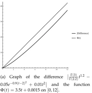
Consider the functiony(t) =t². Then₀^RLD^0.8_t t²= _Γ^Γ₍⁽³⁾

2.2)t^1.2and the inequality

Γ(3) Γ(2.2)^t

1.2−0.05e^{−0.9(t−2)2} +0.01t²

≤3.5t+0.0015 fort∈[0, 12], (6.3) holds (see Figure6.1a).

Consider Φ(t) = 3.5t+0.0015. Then Rt

0(t−s)^−0.2(3.5s+0.0015)ds ≤ _ΛΦ(3.5t+0.0015) withΛΦ =5.5 (see Figure6.1b).

According to Theorem5.7(iii) the solution x(t)of (6.1) satisfies

x(t)−t²

≤39.9618t+0.0199809, t∈ [0, 12]

where c_f = _CΛΦ(1+Q)⁴E_q(0) = 5.5(1.2475)⁴ = 13.3206, C = max_t∈[0,12]E_0.8,0.8(−0.01t^0.8) = 1,Q= (K+L+|b|)CΛ_ΦE_q(_Γ(q)KCτ^q=_0.2475.