Global stability for the 3-dimensional logistic map
János Dudás, Tibor Krisztin University of Szeged, Hungary
February 10, 2020
Abstract. For the delayed logistic equation xn+1 = axn(1− xn−2) it is well known that the nontrivial fixed point is locally stable for 1 < a ≤ √
5 + 1
/2, and unstable for a >
√5 + 1
/2. We prove that for 1 < a≤ √ 5 + 1
/2 the fixed point is globally stable, in the sense that it is locally stable and attracts all points ofS, whereScontains those(x0, x1, x2)∈R3+
for which the sequence (xn)∞n=0 remains in R+. The proof is a combination of analytical and reliable numerical methods. The novelty of this article is an explicit construction of a relatively large attracting neighborhood of the nontrivial fixed point of the 3-dimensional logistic map by using center manifold techniques and the Neimark–Sacker bifurcational normal form.
Keywords: Delayed logistic map; global stability; Neimark–Sacker bifurcation; center mani- fold; interval analysis; rigorous numerics; graph representation
2010 Mathematics Subject Classification: 39A30, 39A28, 65Q10, 65G40, 37C75
1 Introduction
One of the most studied nonlinear maps is the logistic map [0,1] 3 x 7→ ax(1−x) ∈ R with parameter a > 0. It is well known (see e.g., [1]) that x = 0 is the unique fixed point in [0,1]
for 0 < a ≤ 1, and it is globally stable in [0,1]. For 1 < a ≤ 3 the nontrivial fixed point x∗ = 1−1/a is stable and attracts all points of (0,1). Ata = 3 a period doubling bifurcation takes place, and the fixed point x∗ becomes unstable for a > 3. As a increases, there is a sequence of bifurcations, and for some larger value of a, chaotic behavior can be shown.
In 1971 Levin and May [2] considered the delayed logistic difference equation xn+1 =axn(1−xn−d)
with a > 0 and d ∈ N. This is natural in the context of population models; the size of the subsequent generation of the population depends not only on the size in the previous year, but also on the size of the d-year-earlier population.
In cased= 1, it is easy to see that there is a nontrivial positive fixed point fora >1, which is locally asymptotically stable for a∈ (1,2), and unstable fora > 2. In [3] it was shown that this nontrivial fixed point is also globally stable fora ∈(1,2]in the sense that it is locally stable and attracts every point of the set {(u1, u2)∈R2 : u1 ∈[0,1), u2 ∈(0,1), au2(1−u1)<1}.
Bartha, Garab and Krisztin in [4, 5] proved analogous results for other second order dif- ference equations, or equivalently, for other 2-dimensional maps. The novelty of [3, 4, 5] is the development of a new method to show sharp results for global stability of fixed points for some 2-dimensional maps with a parameter a. It is common in [3, 4, 5] that a supercritical Neimark–Sacker bifurcation takes place at some a = acrit. The Neimark–Sacker bifurcational normal form not only guarantees the existence of an invariant curve around the fixed point for
a > acrit, but also for a ≤ acrit it gives a neighborhood M around the fixed point so that M belongs to the region of attraction of the fixed point. The main achievement of [3, 4, 5] is an explicitly constructedMwhich is large enough in the sense that, by using a rigorous computer- assisted technique, it is possible to prove that the iterates of all points outside M eventually enterM. A relatively largeMcan guarantee the success of the computer-assisted part within a reasonable computer time. It is a highly nontrivial result of [3, 4, 5] that starting from the classical Neimark–Sacker bifurcational normal form technique, which was used earlier only for local results, a relatively large attractivity region can be explicitly constructed for a≤acrit. In [3, 4, 5] it was essential that the studied systems were 2-dimensional.
The primary aim of this paper is to extend the method of [3, 4, 5] from 2-dimensional to higher-dimensional maps. As the delayed difference equation is interesting in its own right for d= 2, we study the difference equation
xn+1 =axn(1−xn−2), (1)
which is equivalent to the 3-dimensional map Fa : R3 3u=
u1 u2 u3
7→
u2 u3 au3(1−u1)
∈R3. (2) On this 3-dimensional nonlinear map we demonstrate how the extension goes to higher dimen- sion. We believe that the main steps of our case study for (2) can be followed with natural modifications to handle several other problems, in particular the delayed logistic map ford >2.
Define a0 = √ 5 + 1
/2, and consider the mapFa for those u∈R3+= [0,∞)3 for which all iterates of (2) remain in R3+, i.e., Fan(u) ∈ R3+, for every n ∈ N. Here, Fan denotes the n-fold iteration of Fa, i.e.,Fa0 = id and Fan=Fa(Fan−1), n∈N. As we will see for a∈(0, a0], the set
S˜= ˜S(a) =
u∈R3 : u1, u2, u3 ∈[0,1], au3(1−u1)≤1, a2u3(1−u1)(1−u2)≤1 is the largest set, whose points remain in R3+ for all iterates Fan, n ∈ N. Note that S˜ depends on the parameter a.
For a ∈ (0,1] we have S˜ = [0,1]3, and the only fixed point of (2) in S˜ is the origin. It is elementary to show that the origin is locally stable andlimn→∞Fan(u) = 0for everyu∈S. For˜ a >1 a nontrivial fixed point uA= (A, A, A) with A= 1−1/a appears in S. This fixed point˜ is locally asymptotically stable for a ∈ (1, a0), and unstable for a > a0. A Neimark–Sacker bifurcation takes place at a = a0, and there is a stable invariant curve for a > a0 sufficiently close to a0.
In this paper we show the globally stability of the nontrivial fixed point uA for a ∈(1, a0].
Our main result is the following theorem.
Theorem 1. The fixed point uAis locally stable, and lim
n→∞Fan(u) = uA for every a∈(1, a0]and u∈S(a), where
S(a) =
u∈R3 : u1, u2 ∈[0,1), u3 ∈(0,1), au3(1−u1)<1, a2u3(1−u1)(1−u2)<1 . We emphasize that Theorem 1 is sharp, that is, global stability holds at the critical pa- rameter value a0 as well. Theorem 1 can be formulated so that local stability implies global stability for the fixed point uA. This is satisfied for several problems, see e.g., [6, 7], but it is not true in general (see e.g., [8]). Note that we do not consider the case a > a0. However, local information is available from the Neimark–Sacker bifurcation near uA for a > a0 close to a0. Analogously to the cases d= 0 and d = 1, it is expected that the dynamics becomes more complex with larger a.
In Section 2 we describe the behavior of (2) in the positive octant. Then, for a ∈ (1,4/3]
we give a purely analytical proof of the global stability ofuA. Although this analytical proof is straightforward, it is important toward the proof of Theorem 1, since for a > 1 and close to 1 the fixed point uA can not be distinguished from the origin by a computer-assisted technique.
The rest of the article is devoted to the case a ∈ (4/3, a0]. The basic idea is the same as for the 2-dimensional case. First, we analytically construct an attracting neighborhood M(a) of the fixed point uA. Then, by applying reliable numerical tools, it is shown that for every u ∈ S the iterates Fan(u) eventually enter M(a). Consequently, all points of S belong to the region of attraction ofuA. Here, reliable means that all possible numerical errors are controlled by using interval arithmetic techniques. Therefore, the computer-assisted part also provides mathematically rigorous statements.
In Section 3 the map Fa is transformed to the form Ha : C×R3
z y
7→
λ(a)z+Ga(z, y) ν(a)y+Ha(z, y)
∈C×R (3)
for a ∈ (4/3, a0]. Here, ν(a) ∈ R and λ(a) ∈ C with λ(a)¯ ∈ C are the eigenvalues of the Jacobian matrix of (2) at uA. The inequality |ν(a)| < |λ(a)| ≤ 1 holds and |λ(a0)| = 1. The nonlinear functionsGa(z, y)andHa(z, y)are smooth functions ofa, z,z¯andy, and furthermore, they are O(|(z, y)|2) for each fixed a∈(4/3, a0].
In Section 3.1 a standard linearization technique for (3) gives an attracting neighborhood of uA for a∈ (4/3, a0). When a→ a−0, the attracting neighborhood obtained via linearization shrinks to the fixed point. Therefore, a different approach is necessary for parameter values close to a0. In the subsequent sections, for a ∈ I0 = [a0 −10−2, a0] we adapt the technique from [3, 4] based on the Neimark–Sacker bifurcational normal form. However, we need new ideas, since (2) is 3-dimensional, and thus the adaptation of the method from [3] is not that straightforward.
The classical way to study the dynamics of the 3-dimensional map Fa near uA, or equiva- lently, the dynamics of Ha near (0,0)∈ C×R, for a close to a0 is as follows. First, a center manifold reduction is carried out, then the map is transformed to its normal form on the cen- ter manifold, and finally the attraction property of the center manifold is used. These steps together give a local information on the dynamics of (3) for a is close to a0 and (z, y) is close to (0,0). In particular, for a ≤ a0 and a close to a0, local stability is obtained for the fixed point of (3). The major achievement of this paper is the elaboration of a quantitative version of the above local bifurcation result so that an attractive neighborhood of the fixed point (0,0) can be explicitly constructed. Sections 4–6 are devoted to this issue. In Sections 7 and 8 it turns out that the constructed attracting neighborhood is large enough, and we can handle the remaining points by a rigorous numerical technique.
In Section 4 we consider an approximated version of the center manifold reduction. It is well known that for each fixed a there is a local invariant manifold Wac of map (3) at (0,0) given by the graph
Wac={(z, y)∈C×R: y= Φa(z), |z|< δ}
of a smooth map Φa : {z ∈ C : |z| < δ} → R with some δ = δ(a) > 0 and Φa(0) = 0, Φa(z) = O(|z|2). Note that Φa(·) is not complex differentiable, but it is a smooth function of z and z. The set¯ Wac is a so called generalized center (or center-unstable) manifold of (3) at (0,0)corresponding to the leading eigenvalues λ(a),λ(a)¯ (see [9]). The invariance property of Wac means that Ha(z,Φa(z)) ∈ Wac for z ∈ C with small |z|. Or equivalently, N(Φa(z)) = 0, where N is given by
N(F(z)) =F
λ(a)z+Ga z,F(z)
−ν(a)F(z)− Ha z,F(z) ,
−r r φ(z)
Wac φ(z)−C|z|5
φ(z) +C|z|5
T(r, C)
z 2-dimensional y
Figure 1. The set T(r, C)around the approximation of the center manifold for all maps F :C→R.
The map Φa(z) is problematic concerning its use in quantitative estimations for several reasons. First, it is obtained from a global manifold via modification of the nonlinearity, and its domain can be too small for computational purposes. Furthermore, it is not unique, and there is no explicit formula for it, either. In addition, we need a 3-dimensional attracting set around the fixed point for the computer-aided part, and thus a 2-dimensional set on the manifold is not sufficient. Therefore, we consider a polynomial approximation ofΦa(z), instead.
Namely, for each a∈ I0 there is a unique fourth order (inz,z) polynomial¯ φ(z) = φa(z,z) =¯
4
X
n=2
X
i+j=n
1
i!j!ωij(a)ziz¯j with
N(φ(z)) =O(|z|5).
The advantage ofφ(z)comparing toΦa(z)is that it is defined on the whole complex plane, it is unique, and the coefficientsωij(a)can be easily determined and estimated. The disadvantage is that the graph of φ(z) is not locally invariant under Ha any more. However, a particular 3-dimensional set T containing the graph of y = φ(z) behaves similarly to a center manifold, and in our work it takes over the role of Wac. It will turn out that T is inside the region of attraction of the fixed point.
Define the set
T(r, C) ={(z, y)∈C×R: |z| ≤r, |y−φ(z)| ≤C|z|5}
aroundy =φ(z) (see Figure 1), where r and C are some positive constants. Note thatT(r, C) has a relatively simple form for computational purposes. The term C|z|5 in the definition of T(r, C)guarantees thatT(r, C)contains the invariant manifoldWacfor small|z|. The reason for this special shape of T(r, C), more precisely the termC|z|5, is that the normal form technique needs to be applicable for every (z, y)∈T(r, C).
In Subsections 4.1 and 4.2 we investigate the y-directional dynamics. We use the property that solutions close to the fixed point decay exponentially to T(r, C) since |ν(a)|<|λ(a)| ≤1.
From this it can be shown that T(r, C) is conditionally invariant in direction y for a fixed r, provided that C is sufficiently large. More precisely, for a fixed r and C we show that Ha(T(r, C))⊆T(˜r, C) with some r˜≥r. This means that for(z0, y0)∈ T(r, C) and (z1, y1) =
Ha(z0, y0)∈/T(r, C) we must have|z1|> r, that is, the image under Ha can leaveT(r, C)only in direction z.
In Section 5 thez-directional dynamics is investigated by using the Neimark–Sacker bifurca- tional normal form technique from [3]. For every(z0, y0)∈T(r, C)they-coordinate can be writ- ten in the form y0 =φ(z0) +c|z0|5 for somec∈R with |c| ≤C. Thus, for (z1, y1) =Ha(z0, y0) the z-coordinate is determined by z1 =G(z0), where
G(z) =Ga,c(z,z) =¯ λz+Ga z, φ(z) +c|z|5
. (4)
For a fixed a∈ I0 and c∈Rwith |c| ≤C we can transform (4) into a normal form. Namely, a nonlinear invertible map h:C→C can be given such that
w7→h−1(G(h(w))) =λw+c1w2w+R2(w, w, a, c), (5) where c1 = c1(a, c) is the Lyapunov-coefficient and R2(w, w, a, c) = O(|w|4). It is important (see [3]) that the transformation h is completely determined by the lower order terms of (4).
Because of the special shape of T(r, C), parameter c appears only in the higher order terms of G, i.e., only in R2(w, w, a, c). Consequently, h is independent of c, and w = h(z) can be considered as a coordinate transformation of the whole setT(r, C).
Applying the normal form method from [3], we obtain λw+c1w2w+R2
<|w|
for every sufficiently small w 6= 0. This means that map (5) is a contraction. Consequently, Ha is a contraction in the new w-coordinate. Hence, combining the y- and the z-directional dynamics in Section 5.7, we obtain that T(ˆr, C), with some ˆr < r, is in the region of attraction of the fixed point (0,0)of (3).
However, T(ˆr, C) is clearly not a proper neighborhood of the origin inC×R. Therefore, in Section 6 we define the set
T˜(r, K) ={(z, y)∈C×R: |z| ≤r, |φ(z)−y| ≤K}
for some r > 0 and K > 0. By using the exponential y-directional attractivity of T(r, C) we show that T˜(r, K)is in the region of attraction of the fixed point. The neighborhood T˜ of the fixed point is suitable for the computer-assisted part of the proof.
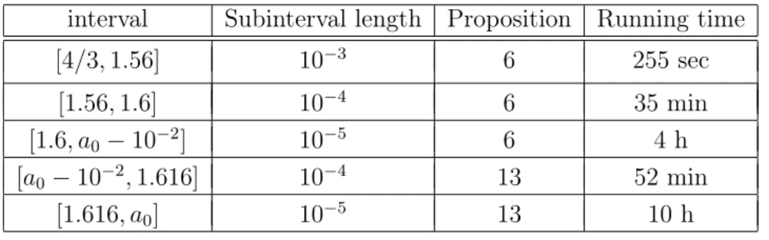
In Sections 7 and 8 we describe the computer-assisted part of our method. We cover S with finitely many small cubes. Considering these cubes as vertices of a graph we introduce a directed graph, which, to a certain extent, describes the behavior of map (2) on these cubes. Therefore, we convert the issue of examining infinitely many points into a finite graph problem, which can be handled by computer. To construct the edges of this graph we use reliable numerical methods in order to handle the rounding errors of the computer. We show with the help of this graph that the iterates of every point from S(a) enter the neighborhood constructed before, and the proof of Theorem 1 is completed.
Despite the fact that we demonstrate our method only on a specific equation, we believe that it can be applied or extended to other similar maps. For instance the Ricker map (see [4]) and the Pielou map (see [10]) with delay d = 2 essentially differs only in that they are not polynomial maps. Hence, only a slight modification would be necessary in the estimations.
However, the main question is whether the obtained neighborhood is large enough for the computer-aided part of the method. These two maps along with the logistic map would also be interesting for larger delay, i.e., d >2. We believe that the analytical part could be extended using only natural modifications. However, the computer-aided part can be critical in these cases, since the increasing dimension causes exponentially growing graph.
It also would be interesting to prove the existence of the unique invariant closed curve around the nontrivial fixed point for parameter values larger than the critical value. However, this question is substantially different from the one studied in this article.
2 Preliminaries
Throughout the articleN,N0 andR+denote the positive integers, the nonnegative integers and the nonnegative real numbers, respectively. We use also the big O notation in the sense that f(x) = O(g(x)) means that there exist positive numbers δ and M such that |f(x)| ≤ M g(x) for |x|< δ.
For symbolic computation we use Wolfram Mathematica v. 11, and for reliable numerical estimation we use interval arithmetic tools of IntLab v. 9 in Matlab 2018.
In this section we study the dynamics of map (2) in the positive octant fora >0. Introduce the following disjoint sets depending on a (see Figure 2).
S =
u∈R3 : u1, u2 ∈[0,1), u3 ∈(0,1), au3(1−u1)<1, a2u3(1−u1)(1−u2)<1 S˜0 ={(u1, u2,0) : u1, u2 ≥0}
∪{(1, u2, u3) : u2 ≥0, u3 >0}
∪{(u1,1, u3) : u1 ∈[0,1), u3 >0}
∪{(u1, u2,1) : u1, u2 ∈[0,1)}
∪{(u1, u2, u3) : u1, u2 ∈[0,1), u3 ∈(0,1), au3(1−u1) = 1}
∪
(u1, u2, u3) : u1, u2 ∈[0,1), u3 ∈(0,1), au3(1−u1)<1, a2u3(1−u1)(1−u2) = 1 S˜1 =
(u1, u2, u3) : u1, u2 ∈[0,1), u3 ∈(0,1), au3(1−u1)<1, a2u3(1−u1)(1−u2)>1 S˜2 ={(u1, u2, u3) : u1, u2 ∈[0,1), u3 ∈(0,1), au3(1−u1)>1}
S˜3 ={(u1, u2, u3) : u1, u2 ∈[0,1), u3 >1}
S˜4 ={(u1, u2, u3) : u1 ∈[0,1), u2 >1, u3 >0}
S˜5 ={(u1, u2, u3) : u1 >1, u2 ≥0, u3 >0}
Clearly,R3+=S∪S˜0∪S˜1∪S˜2∪S˜3∪S˜4∪S˜5. Furthermore,S = [0,1)2×(0,1)andS˜1 = ˜S2 =∅ for 0< a≤1. Introduce the notation uˆ=Fa(u) with uˆ= (ˆu1,uˆ2,uˆ3).
Proposition 2. For all a >0 and i∈ {1,2,3,4} we have
Fa7( ˜S0) = {(0,0,0)}, Fa( ˜S5)∩R3+ =∅ and Fa( ˜Si)⊆S˜i+1. Furthermore, Fa(S)⊆S for a∈(1, a0].
Proof. From the definition of Fa it is obvious that Fa7( ˜S0) = {(0,0,0)}. It is also straightfor- ward to check the relations Fa( ˜S5)∩R3+ =∅ and Fa( ˜Si)⊆S˜i+1 for i∈ {1,2,3,4}.
If u∈S then uˆ=Fa(u)satisfies ˆ
u1 =u2 ∈[0,1), uˆ2 =u3 ∈(0,1), uˆ3 =au3(1−u1)∈(0,1) and
aˆu3(1−uˆ1) =a2u3(1−u1)(1−u2)<1. (6) For the last inequality in the definition of S we have
a2uˆ3(1−uˆ1)(1−uˆ2) =a3u3(1−u1)(1−u2)(1−u3).
Foru3 ≥A = 1−1/a it follows from (6) that
a2uˆ3(1−uˆ1)(1−uˆ2) = a a2u3(1−u1)(1−u2)
(1−u3)< a(1−u3)≤1.
Foru3 < A, provided that a∈(1, a0], we obtain
a2uˆ3(1−uˆ1)(1−uˆ2)≤a3u3(1−u3)< a3A(1−A) = a2−a≤1,
1 a
1−a1 1
S˜5 S˜4
S˜3
S˜2
S˜1 S
u1 u2
u3
Figure 2. The subdivision of the positive octant since A≤1/2. Thus, Fa(S)⊆S.
Consequently, in the rest of the paper we can assume thatu∈S. For smallathe dynamics in Sis simple. The following statement easily follows from the fact thatxn+1 =axn(1−xn−2)< xn, provided that xn−2, xn∈(0,1]and 0< a≤1.
Proposition 3. For every 0< a≤1 and u∈[0,1]3 the following holds
n→∞lim Fan(u) = (0,0,0).
For a ∈ (1, a0] we divide S into eight subsets with planes u1 = A, u2 = A, u3 = A, and introduce the following sets.
S1 ={u∈S : u1 ≤A, u2 ≤A, u3 < A}
S2 ={u∈S : u1 < A, u2 > A, u3 < A}
S3 ={u∈S : u1 ≥A, u2 > A, u3 ≤A}
S4 ={u∈S : u1 > A, u2 ≤A, u3 ≤A}
S5 ={u∈S : u1 ≤A, u2 < A, u3 ≥A}
S6 ={u∈S : u1 < A, u2 ≥A, u3 ≥A}
S7 ={u∈S : u1 ≥A, u2 ≥A, u3 > A}
S8 ={u∈S : u1 > A, u2 < A, u3 > A}
Clearly, S =S8
i=1Si∪ {uA}. For given x0, x1, x2 the sequence (xn)∞n=0, where xn is defined by (1) for n >2, corresponds to the 3-dimensional sequence(un)∞n=0 with
u0 = (x0, x1, x2), un =Fan(u0) = (xn, xn+1, xn+2), n ∈N.
S1
S2
S3 S4
S5
S6
S7
S8
x y
z
Figure 3. The dynamics in S\uA. The sets Si are symbolized by a smaller cube, for the sake of transparency.
Proposition 4. Let a ∈ (1, a0] and the sequence (un)∞n=0 in S be given by u0 6= uA and un=Fan(u0), n∈N.
(i) The sequence (un)∞n=0 follows the transition graph given in Figure 3.
(ii) If(un)∞n=0 does not converge touAthen there exists ann0 ∈Nsuch thatun0 ∈S1, (un)∞n=n0 follows the transition graph
S1 S5 S6 S7 S3 S4
and (un)∞n=n0 does not eventually stay in S1 or S7.
Proof. In order to show (i), observe the following transitions, see Figure 3.
◦ For u ∈ S1 we obtain uˆ = Fa(u) with uˆ1 ≤ A and uˆ2 < A. Therefore, S1 {S1, S5}, that is, uˆ∈S1 or uˆ∈S5.
◦ Foru∈S2 we have uˆ1 > A and uˆ2 < A. Thus, S2 {S4, S8}.
◦ Foru∈S3 we get uˆ1 > A, uˆ2 ≤A and uˆ3 =au3(1−u1)≤aA(1−A) = A, so S3 S4.
◦ Foru∈S4 we have uˆ1,uˆ2 ≤A and uˆ3 < A. Consequently, S4 S1.
◦ Foru∈S5 we obtain uˆ1 < A, uˆ2 ≥A and uˆ3 ≥A. Hence, S5 S6.
◦ Foru∈S6 we get uˆ1,uˆ2 ≥A and uˆ3 > A. Consequently, S6 S7.
◦ Foru∈S7 we have uˆ1 ≥A and uˆ2 > A. Therefore, S7 {S3, S7}.
◦ Foru∈S8 we have uˆ1 < A and uˆ2 > A, so S8 {S2, S6}.
We obtain that there is a cycleC1 = (S1 S5 S6 S7 S3 S4 S1). If a sequence (un)∞n=0 enters the cycle C1 then the sequence never leavesC1. However, during one cycle along C1, the points of(un)∞n=0 can spend more time inS1 orS7. Possibly, the sequence can get stuck and stay forever in S1 or S7. Furthermore, we have another cycle C2 = (S2 S8 S2). If a sequence steps out of the cycle C2 then it enters C1 and never returns to C2. Consequently, we only need to show that if a sequence (un)∞n=0 gets stuck in S1 or S7, or in the cycle C2 then it converges to the fixed point uA.
First, consider the case, when the sequence (un)∞n=0 stays in C2. We can assume x0 < A.
We obtain a sequence (xn)∞n=0 such that x2k < Aand x2k+1 > A, where k∈N0. Since A < x2k+1 =ax2k(1−x2k−2) = 1
1−Ax2k(1−x2k−2), we get
A(1−A)< x2k(1−x2k−2). (7) Introduce the function s(x) = x(1−x). Since s(x) is increasing on [0,1/2] and 0 ≤ x2k−2 <
A <1/2we obtain s(x2k−2)< s(A). Combining it with (7) we get x2k−2 < x2k. Consequently, (x2k)∞k=0 converges monotonically to some B ≤A. Taking the limit of both sides in inequality (7), we obtain A(1−A) ≤ B(1− B). On the other hand s(x) is increasing on [0, A], so B(1−B) ≤ A(1−A). Thereby B = A. The odd indexed subsequence also converges to A, sincex2k+1 =ax2k(1−x2k−2)→aA(1−A) = A. So in this case, the sequence(un)∞n=0 converges to the nontrivial fixed point uA.
Now, consider the case, when the sequence gets stuck inS1, i.e., there exists ann0 ∈N0 such that (un)∞n=n0 is in S1. Notice that un ∈S1 implies xn+2 ≤xn+3, since xn ≤ A. Consequently, we gain a monotone, bounded sequence (xn)∞n=n0+2 which converges to some B ≤ A. Taking the limit of both sides in (1), we obtain B =A. Consequently, the point u0 is in the region of attraction of uAin this case. Similarly, if(un)∞n=0 gets stuck in S7, it also converges to the fixed point uA.
Now, we assume1< a≤4/3, and show that for everyu0 ∈Sthe sequence(un)∞n=0converges to the nontrivial fixed point uA. Combining this fact with the local asymptotic stability of the fixed point (see Section 3), Theorem 1 is proven for these parameter values.
Proposition 5. If a∈(1,4/3] and u∈S, then lim
n→∞Fan(u) = uA.
Proof. It follows from Proposition 4 that we only need to consider the case when the sequence (un)∞n=0 goes around the fixed point along the cycle C1, not getting stuck in S1 or S7. By the definition of S and Fa(S) ⊆ S we obtain xn >0 for all n ≥ 2. Without loss of generality we can assume that u0 ∈ S1, x0 >0 and x1 >0. Then xn >0 for all n ∈ N0. There is a strictly increasing subsequence (nl)∞l=0 of N0 such thatn0 = 0, un2k ∈S1 and un2k+1 ∈S7 with
uj ∈/ S7 for j ∈ {n2k, . . . , n2k+1−1}, uj ∈/ S1 for j ∈ {n2k+1, . . . , n2k+2−1}.
Note thatnl+1−nl ≥3holds (see the transition graph in Figure 3). Furthermore, the definition of (nl)∞l=0 implies
xj ≤A for j ∈ {n2k, . . . , n2k+1−1},
xj ≥A for j ∈ {n2k+1, . . . , n2k+2−1}. (8) From (1) and xn >0, n∈ N0 it is clear that xn−2 ≤A if and only if xn ≤xn+1. Combining it with (8) we obtain (xj)nj=n2k+1+2
2k+2 is nondecreasing and (xj)nj=n2k+2+2
2k+1+2 is nonincreasing.
For the function t: [0,1]3x7→a2(a−1)(1−x)3 ∈R we have t(A) =A and d
dxt(x) = −3a2(a−1)(1−x)2 ≤0, d2
dx2t(x) = 6a2(a−1)(1−x)≥0, d
dxt(t(x)) = 9a4(a−1)2 1−t(x)2
(1−x)2 ≥0, d2
dx2t(t(x)) = 18a4(a−1)2(1−x) 1−t(x)
4t(x)−1 .
Forx∈(A,1]we obtain4t(x)−1<4A−1≤0, provided thata ∈[1,4/3]. Hence, dxd22t(t(x))<0 for allx∈(A,1). Furthermore, dxdt(t(x))
x=A = 9(a−1)2 ≤1fora∈ 1,43
. Thus, dxdt(t(x))<1 for all x∈(A,1). Therefore, the only fixed point of [A,1]3x7→t(t(x))∈R isA.
Let (sk)∞k=0 be given by s0 = 0 and sk = tk(s0) for k ∈ N. Clearly, (s2k)∞k=0 is strictly increasing with s2k < A for k ∈ N0 and (s2k+1)∞k=0 is strictly decreasing with s2k+1 > A for k ∈N0. We have
xj ≥s0 for j ∈ {n0, . . . , n1−1}.
Suppose
xj ≥s2k for j ∈ {n2k, . . . , n2k+1−1}.
Then using (8) we obtain
xn2k+1+2 =axn2k+1+1(1−xn2k+1−1) =a2xn2k+1(1−xn2k+1−1)(1−xn2k+1−2)
=a3xn2k+1−1(1−xn2k+1−3)(1−xn2k+1−2)(1−xn2k+1−1)≤a3A(1−s2k)3 =s2k+1. Similarly,
xj ≤s2k+1 for j ∈ {n2k+1, . . . , n2k+2−1}
implies
xn2k+2+2 =axn2k+2+1(1−xn2k+2−1) =a2xn2k+2(1−xn2k+2−2)(1−xn2k+2−1)
=a3xn2k+2−1(1−xn2k+2−3)(1−xn2k+2−2)(1−xn2k+2−1)≥a3A(1−s2k+1)3 =s2k+2. It follows that
xj ∈[s2k, A] for j ∈ {n2k, . . . , n2k+1−1}, xj ∈[A, s2k+1] for j ∈ {n2k+1, . . . , n2k+2−1}
for all k ∈N0. Clearly, sk →A impliesxk →A.
As (s2k+1)∞k=0 is a decreasing sequence in [A,1], s2k+3 =t(t(s2k+1)), and A is the only fixed point of t(t(x)) in [A,1], we obtain s2k+1 →A. The continuity oft and s2k+2 =t(s2k+1) gives s2k→A.
We remark that the technique of [11, 7] seems to work for (1) to get global stability for 1 < a < 14/9. However, [11, 7] does not apply directly, some additional work is necessary.
Note that Proposition 5 is essential in the sense that the case a≈1 can not be handled in the computer-aided part of the method. The two fixed points can be arbitrarily close to each other, so after some point they can not be handled efficiently by interval arithmetic tools. Moreover, if they get closer to each other, they can not even be distinguished in the floating point system.
In the rest of the paper we assume a∈(4/3, a0].
3 An attracting neighborhood with linearization
For each fixed a, translating uA into0∈R3, i.e., introducing the new variable v =u−uA, the shifted version
R3 3v 7→Fa(v+uA)−uA∈R3 of (2) can be written as
R3 3v 7→Jav+fa(v)∈R3, (9) where
Ja =
0 1 0
0 0 1
1−a 0 1
, fa(v) =
0 0
−av1v3
. The characteristic polynomial of Ja is
P(a, λ) =−λ3 +λ2 + 1−a,
and the roots of P(a, λ) are λi = λi(a), where i ∈ {0,1,2}. Since P(1, λ) = −λ2(λ −1) and P(31/27, λ) = −(λ+ 1/3) (λ−2/3)2, it follows from the graph of P(a, λ) that for a ∈ (1,31/27] the polynomial P(a, λ) has three real roots (counting multiplicity) and |λi| < 1 for i ∈ {0,1,2}. For a > 31/27 the characteristic polynomial has a real root ν = ν(a) = λ0 and two complex roots λ1 = ¯λ2. Denote λ the complex root with positive imaginary part, i.e., λ=λ(a) = λ1. Formulas of ν and λ can be found in the Appendix, see Section 10.1.
From the graph of P(a, λ) it follows that ν < 0 and ν is a strictly decreasing function of a for a > 31/27. Since P(3, λ) = −(λ+ 1)(λ−1−i)(λ−1 +i), it is clear that |ν| < 1 for a∈(31/27,3). From Vieta’s formulas it follows that
ν+ 2 Reλ = 1, 2νReλ+|λ|2 = 0, ν|λ|2 = 1−a.
From the first two formulas we get
|λ|2 =ν2 −ν. (10)
Combining the facts thatR3s 7→s2−s∈Ris decreasing on(−∞,0], andν(a)is a decreasing function of a, we obtain |λ(a)| is a strictly increasing function of a. From (10) and the third Vieta’s formula, it follows that |λ|= 1 implies ν = 1−√
5
/2 and a =a0. Thus, we obtain for a ∈ (1, a0) that |λi| < 1, i ∈ {0,1,2}, i.e., the fixed point uA of Fa is locally stable. For a > a0 we get |λ|>1, so the fixed point is unstable.
The eigenvectors qi, corresponding to the eigenvalues λi of Ja, are qi = qi(a) = (1, λi, λ2i), i∈ {0,1,2}. Let Qa be the matrix, whose columns are the eigenvectors qi, i.e.,
Qa =
1 1 1
λ λ¯ ν λ2 ¯λ2 ν2
.
For a >31/27the matrix Qa is invertible and
Q−1a =
d(λ2−λ) d(λ−1) d d¯ λ¯2−λ¯ d¯ λ¯−1 d¯
e(ν2−ν) e(ν−1) e
, (11) where
e=e(a) = 1
3ν2 −2ν, d=d(a) = 1 3λ2 −2λ. Note that the rows of Q−1a are the eigenvectors of JaT.
Applying the linear transformation Z =
z
¯ z y
=Q−1a
v1 v2 v3
, the map (9) takes the following form
Z 7→Q−1a JaQaZ+Q−1a fa QaZ
=
λ z+d g(z, y)
¯λz¯+ ¯d g(z, y) ν y+e g(z, y)
, (12) where the function g :C×R→R is
g(z, y) =ga(z,z, y) =¯ −a(z+ ¯z+y) λ2z+ ¯λ2z¯+ν2y
. (13)
Clearly, the second component in (12) is the complex conjugate of the first one. Therefore, it is sufficient to consider the map
Ha: C×R3 z
y
7→
λz+d g(z, y) νy+e g(z, y)
∈C×R. (14)
Remark that for the sake of simplicity, we omit the argumentz, and indicate only variable¯ z in the subsequent functions. We also emphasize that g(z, y) andHa(z, y) are smooth functions of z,z¯and y, but they are not necessarily complex differentiable.
3.1 Local stability by linearization
First, for a fixed parameter a ∈ (4/3, a0) we use the map (14) without further transformation to construct a neighborhood M0(a) ⊆ C×R, which is inside the region of attraction of the origin, i.e., limn→∞Han(z, y) = (0,0) for every (z, y)∈ M0(a).
Proposition 6. For every a∈(4/3, a0) define ξ(a) by ξ(a) = (1− |λ|)
4a|λ|2(|d|+|e|). Then the set
M0(a) ={(z, y)∈C×R: |z|+|y|< ξ(a)}
is in the region of attraction of the fixed point (0,0) of Ha.
Proof. Introduce the norm |(z, y)|=|z|+|y| on the space C×R. We show that there exists a ξ = ξ(a) > 0 such that |Ha(z, y)| < |(z, y)| for every 0 < |(z, y)| < ξ. If such a ξ exists, it is clear that the open ball Bξ◦ around the origin is invariant. We show that every point of Bξ◦ tends to the origin. Let (z0, y0) be an arbitrary point from Bξ◦ and consider the nonnegative, strictly decreasing sequence (|(zn, yn)|)∞n=0, where (zn+1, yn+1) = Ha(zn, yn). This sequence can converge only to a fixed point of the continuous map r 7→ max|(z,y)|=r|Ha(z, y)|, which is only r= 0, provided that r∈[0, ξ).
From (10) we obtain |λ|>|ν|for 4/3< a < a0, so
|g(z, y)| ≤4a|λ|2(|z|+|y|)2 = 4a|λ|2|(z, y)|2. Consequently, estimating (14) we obtain
|Ha(z, y)| ≤ |λ||(z, y)|+ (|d|+|e|)|g(z, y)|
≤ |(z, y)| |λ|+ (|d|+|e|) 4a|λ|2|(z, y)|
<|(z, y)|
for every (z, y)6= (0,0), provided that |(z, y)|< ξ(a), where ξ(a) = 1− |λ|
4a|λ|2(|d|+|e|). Therefore,ξ(a) is a suitable choice.
First, note that M0(a) is in C×R. Clearly, this set corresponds to an attracting neigh- borhood M(a) ⊆ R3 around the nontrivial fixed point uA of (2). However, we let this trans- formation be done in the second, computer-aided part of the proof, in order to obtain better accuracy.
Second, since lima→a0|λ(a)| = 1, we obtain M0(a) shrinks to the origin as a tends to a0. However, the smaller the neighborhood is, the less efficient and more time-consuming the computer-aided part of the proof is. Furthermore, Proposition 6 does not provide at all an attractive neighborhood at the critical parameter value a0. Consequently, close to a0 this approach is not suitable for reliable numerical methods, and thus we need to find another way to construct the attracting neighborhood.
4 A center manifold reduction
In the subsequent sections we study the case a ∈ I0 = [a0 −10−2, a0]. For a ∈ I0 we want to adapt the normal form technique from [3] to create an attracting neighborhood around the nontrivial fixed point of map (2). However, map (2) is 3-dimensional, so we need a center manifold reduction first (see [12, 13, 14]).
As we explained in the Introduction, a polynomial approximation of the generalized center- unstable manifold will be used here for each a ∈ I0. We look for the fourth order polynomial approximation φ(z) = φa(z,z)¯ of the manifold in the form
φ(z) =
4
X
n=2
X
i+j=n
1
i!j!ωijziz¯j, (15) where ωij =ωij(a). Every coefficient ωij is determined so that in the expression
N(φ(z)) = φ
λz+d g z, φ(z)
−νφ(z)−e g z, φ(z)
(16) the at most fourth order terms of z,z¯ are eliminated (see [13]), so N(φ(z)) = O(|z|5). The coefficients ωij depend smoothly on a and the formulas can be found in the Appendix, see Section 10.3. In the subsequent sections we study the dynamics of (14) in the set
T(r, C) = {(z, y)∈C×R: |z| ≤r, |y−φ(z)| ≤C|z|5}.
Note that it would suffice to consider a second order approximation of the generalized center- unstable manifold with a term C|z|3 in T(r, C) in order to obtain an attracting neighborhood.
Also in this case C would appear only in the at least fourth order terms of (4) which is of crucial importance. However, this does not provide a sufficiently large neighborhood for the computer-aided part of the method. Indeed, the larger the order of the approximation of the center manifold is, the larger the obtainable initial attracting neighborhood is, since our estimates are more precise. On the other hand, calculations become lengthier as the order of the approximation increases. Furthermore, the growth of attracting neighborhood due to extra orders is diminishing, that is why, we have chosen a fourth order approximation for φ(z).
Throughout the article we need an a-independent estimate of some coefficients. First of all, it is easy to see that
|λ| ≤1 and |ν| ≤ν0 for a∈ I0, (17) where ν0 =a0−1. Furthermore, with interval arithmetic it can be shown that d0 = 0.559 and e0 = 0.425 satisfy the inequalities
|d| ≤d0 and |e| ≤e0 for a∈ I0. (18) Then, we choose constants ωk, k∈ {2,3,4} such that the following holds
X
i+j=k
|ωij|
i!j! ≤ωk for a∈ I0.
With interval arithmetic we obtain that ω2 = 1.29, ω3 = 2.193 and ω4 = 6.233 are appropriate choices. Letφk(z) denote the k-th order terms of φ(z). We obtain
|φk(z)| ≤ωkrk (19)
for k ∈ {2,3,4}and a∈ I0. Clearly, (19) implies the polynomial estimate
|φ(z)| ≤φmax(|z|) (20)
for every a∈ I0, where
φmax(r) =
4
X
k=2
ωkrk
is a real polynomial with positive coefficients. However, estimate (19) is a stronger property than merely (20). We refer to an estimate like (20) as an estimate by order, if inequalities similar to (19) also holds.
Now, we turn our attention to the function g(z, y) from (13) and consider the expansion g(z, y) = X
i+j+k=2
gijk
i!j!k!ziz¯jyk, (21) where
gijk =gijk(a) =−a iλ2+j¯λ2+kν2 .
Using interval arithmetics it can be shown that g20 = 4.237, g11 = 3.805 and g02 = 0.6181 satisfy
X
i+j=2
|gij0|
i!j! ≤g20, X
i+j=1
|gij1|
i!j! ≤g11, |g002|
2! ≤g02 for a∈ I0. Thus, from (21) we obtain
|g(z, y)| ≤g˜max(|z|,|y|) (22) for every a∈ I0, where
˜
gmax(r, s) = g20r2+g11rs+g02s2.
Here, we also estimate by order (distinguishingyfromz andz, but handling¯ z and z¯together), and the coefficients of the second order polynomial gmax(r, s) are positive.
Later, we need also the composition of functions φ and g, so we introduce the 8th order polynomial
gmax(r) = ˜gmax r, φmax(r) ,
and for every a ∈ I0 we obtain
|g(z, φ(z))| ≤gmax(|z|). (23) It is important that (23) is also an estimate by order, since it is a composition of two functions with that property.
After these estimations we can proceed to show the conditional invariance of T(r, C). First of all, y = φ(z) is just an approximation of the center manifold, so N(φ(z)) is not zero.
Nevertheless, N(φ(z)) = O(|z|5) follows from the choice of coefficients ωij. In the computer- aided part, for a given ρ1 >0 we need an explicitN(φ(z))≤C0|z|5-type estimate for|z| ≤ ρ1 and a∈ I0, where the constant C0 is independent of a and z.
Proposition 7. Letρ1 = 0.02234andC0 = 37.379. For every|z| ≤ρ1 anda∈ I0 the following holds
|N(φ(z))| ≤C0|z|5.
Proof. Because of the construction of φ(z), the fourth and lower order terms of z,z¯are zero in (16). To gain a better estimate ofC0, we consider the decomposition
N(φ(z)) = N5(z) +N≥6(z),
whereN5(z)andN≥6(z)denote the fifth and the at least sixth order terms ofN(φ(z)), respec- tively. Clearly, N5(z)can be written in the following form
N5(z) = X
i+j=5
Nij i!j!ziz¯j,
where Nij = Nij(a). Using (15) and (21) the coefficients Nij can be determined explicitly for i+j = 5. The formulas can be found in the Appendix, see Section 10.4. With interval arithmetic it can be shown that N5 = 25.094 satisfies
X
i+j=5
|Nij|
i!j! ≤N5 (24)
for every a∈ I0. From this we obtain |N5(z)| ≤N5|z|5 for a∈ I0.
For the estimation of N≥6(z) we use (17), (18), (20) and (23). For every a∈ I0 we get
|N(φ(z))| ≤φmax r+d0gmax(r)
+ν0φmax(r) +e0gmax(r), (25) where r=|z|. The right hand side of (25) is a polynomial, so it can be written in the form
φmax r+d0gmax(r)
+ν0φmax(r) +e0gmax(r) =
32
X
k=2
b0,krk.
Thea-independent real coefficientsb0,k can be determined by the real polynomials φmax(r)and gmax(r). The inequality (25) is also an estimate by order, since (20) and (23) also have that property. Furthermore, the lower order terms ofN(φ(z))were eliminated, so the following also holds
|N≥6(z)| ≤
32
X
k=6
b0,krk.
Note that this inequality would not be necessarily true without the estimate of order property.
Using r≤ρ1 we obtain
|N≥6(z)| ≤
32
X
k=6
b0,kρk−51
!
|z|5.
It can be show that N6 = 12.285 satisfies
32
X
k=6
b0,kρk−51 ≤N6. (26)
Combining (24) and (26) we obtain
|N(φ(z))| ≤ |N5(z)|+|N≥6(z)| ≤(N5+N6)|z|5. So the proposition is proven, since C0 was chosen such that N5+N6 ≤C0.
In the following corollary we reformulate Proposition 7 in order to obtain a geometrical interpretation of the statement (see Figure 4).
Corollary 8. Let ρ1 and C0 be from Proposition 7. For every |z0| ≤ ρ1 and a ∈ I0 the point (ˆz0,yˆ0) =Ha(z0, φ(z0))satisfies the inequality
|φ(ˆz0)−yˆ0| ≤C0|z0|5.
4.1 Attractivity in direction y
Corollary 8 states that for parameter values close to the critical a0 if we consider a point (z0, y0) from the surface (z, φ(z)), i.e., y0 = φ(z0), then the image (ˆz0,yˆ0) remains close to that surface. Now, with the help of Corollary 8 we are able to make a statement about the y-directional behavior of map (14). It is well-known (see [14]) that if the fixed point has no eigenvalues moduli greater than one, then the center manifold has an attracting property, i.e., every solution close enough to the fixed point decays exponentially to the center manifold.
Based on this idea we prove a similar statement about the approximation y = φ(z) of the center manifold.
Proposition 9. Let ρ1 and C0 be from Proposition 7. Furthermore, let ρ˜2 = 0.0237, σ = 2.1·10−3 and L= 0.66. For every |z0| ≤ρ1, |y0| ≤σ and a∈ I0 the point (z1, y1) =Ha(z0, y0) satisfies |z1| ≤ρ˜2 and
|φ(z1)−y1| ≤L|φ(z0)−y0|+C0|z0|5.
Proof. First, note that σ was chosen large enough such that Proposition 9 can be applied in Propositions 10, 12 and 13, i.e., {(z, y)∈C×R: |z| ≤ρ1, |y| ≤σ} contains the occurring T and T˜. Second, from (14), (17), (18) and (22) it is clear that
|z1| ≤ |z0|+d0g˜max(|z0|,|y0|) for every a∈ I0. The constant ρ˜2 was chosen such that
˜
ρ2 ≥ρ1+d0g˜max(ρ1, σ).
Thus, we obtain that |z1| ≤ ρ˜2 for every |z0| ≤ ρ1 and |y0| ≤ σ. Similarly, |ˆz0| ≤ ρ˜2 also holds for (ˆz0,yˆ0) =Ha(z0, φ(z0)), since φmax(ρ1) ≤ σ (see Corollary 8 and Figure 4). Finally, introducing the notation ki =yi−φ(zi) for i∈ {0,1} (see Figure 4), the formula to be proven in this proposition can be reformulated into the form
|k1| ≤L|k0|+C0|z0|5. Using (14) and the mean value theorem we obtain
z1 =λz0+d g z0, φ(z0) +k0
= ˆz0+d k0∂2g z0, φ(z0) + ˜k0 , y1 =ν φ(z0) +k0
+e g z0, φ(z0) +k0
= ˆy0+ν k0+e k0∂2g z0, φ(z0) + ˆk0
, (27)