A study of logistic growth models influenced by the exterior matrix hostility
and grazing in an interior patch
Nalin Fonseka, Jonathan Machado and Ratnasingham Shivaji
BUniversity of North Carolina at Greensboro, Department of Mathematics and Statistics, Greensboro, NC 27412, USA
Received 31 August 2019, appeared 18 March 2020 Communicated by Péter L. Simon
Abstract.We will analyze the symmetric positive solutions to the two-point steady state reaction-diffusion equation:
−u00=
λ
u− 1
Ku2− cu
2
1+u2
; x∈[L, 1−L],
λ
u− 1 Ku2
; x∈(0,L)∪(1−L, 1),
−u0(0) +√
λγu(0) =0, u0(1) +√
λγu(1) =0,
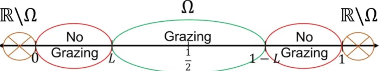
whereλ,c,K, andγare positive parameters and the parameter L∈(0,12). The steady state reaction-diffusion equation above occurs in ecological systems and population dynamics. The above model exhibits logistic growth in the one-dimensional habitat Ω0= (0, 1), where grazing (type of predation) is occurring on the subregion[L, 1−L]. In this model, u is the population density and cis the maximum grazing rate. λis a parameter which influences the equation as well as the boundary conditions, andγrep- resents the hostility factor of the surrounding matrix. Previous studies have shown the occurrence of S-shaped bifurcation curves for positive solutions for certain parameter ranges when the boundary condition is Dirichlet (γ −→ ∞). Here we discuss the oc- currence of S-shaped bifurcation curves for certain parameter ranges, whenγis finite, and their evolutions asγand Lvary.
Keywords: differential equations, boundary value problems, logistic growth, exterior matrix hostility, interior grazing, positive solutions.
2020 Mathematics Subject Classification: 34B08, 34B15, 34B18.
BCorresponding author.
Emails: g_fonsek@uncg.edu (N. Fonseka), jonathan.Machado@tufts.edu (J. Machado) r_shivaj@uncg.edu (R. Shivaji)
1 Introduction
First, we briefly discuss the history of grazing type models. Recently in [5], authors discussed the following boundary value problem:
−∆u=λ
u− u
2
K − cu
2
1+u2
; Ω,
∂u
∂η+√
λu=0; ∂Ω,
(1.1)
where ∂u∂η is the outward normal derivative ofu,λ>0,K >0, 0<c<2, andΩis a bounded domain in RN; N ≥ 1 with smooth boundary ∂Ω. Here, u is the population density, λ is a positive parameter, and c is the maximum grazing rate. The term u− K1u2 represents a logistic growth, which means the per capita growth rate is a linear depreciation. The term
cu2
1+u2 represents the rate of grazing by a constant number of grazers (see Figure 1.2). The authors established the occurrence of S-shaped bifurcation curves when parameters cand K satisfy certain conditions. Grazing type models apply to many ecological systems arising in population dynamics such as the dynamics of salmon fish and spruce budworms (see [9] and [12]).
Figure 1.1: Examples of salmon and spruce budworms
However, it turns out that the grazing presents itself only in an interior patch in many real-world situations. We refer the reader to [1] for a study in this direction where the authors studied the following Dirichlet boundary value problem:
−u00 = (
λf˜(u); x ∈[L, 1−L],
λf(u); x ∈(0,L)∪(1−L, 1), u(0) =u(1) =0,
(1.2)
where ˜f(u) = u− K1u2− 1cu+u22 and f(u) = u− K1u2, which corresponds to the case where γ→∞(see (1.5)). Now,λ,c, andKare positive parameters and the parameter L∈(0,12). The authors showed the occurrence of S-shaped bifurcation curves for certain parameter ranges and numerically obtained the evolution of the bifurcation curves over a range ofL-values and K-values, for a fixed value of c. In particular, for c = 1.5 they showed that occurrence of S-shaped bifurcation persists for any value ofL, ifKis chosen to be large enough.
Biologists have recently observed that in the study of grazing models, to better predict the behavior of the ecological system, it is vital to take the exterior matrix hostility factor into
Figure 1.2: Grazing.
account. In this paper, we extend the study in [1] to the case when the exterior matrix hostility is incorporated into the model. We obtain our results via a modified quadrature method and Mathematica computations.
We now briefly discuss the modeling aspect of the problem. We consider the domain Ω0 ={lx|x ∈Ω}, whereΩ= (0, 1)andlis a parameter representing the size of the habitat.
We assume that the diffusion rate in the patchΩ0isD. In the matrixR\Ω0, we assume that the diffusion rate isD0, and the death rate isS0.
We will further assume that the population exhibits density dependent dispersal (DDD) on the boundary ∂Ω0. Defining α(u) as the probability of the population remaining in Ω0
when it reaches the boundary, the resulting model is (see [2,6,10,11]):
ut= Duxx+h(u); x∈Ω0,t>0, u(0,x) =u0(x); x∈Ω0, Dα(u)∂u
∂η +
√S0D0
k [1−α(u)]u=0; x∈∂Ω0,t>0
(1.3)
with the corresponding steady state equation:
−u00 = 1
Dh(u); x∈ Ω0,
Dα(u)∂u
∂η +
√S0D0
k [1−α(u)]u=0; x∈ ∂Ω0, or equivalently
−u00 = l
2
Dh(u); x∈ Ω,
∂u
∂η +
√S0D0l kD
1−α(u) α(u)
u=0; x∈ ∂Ω,
(1.4)
where kis a positive parameter related to the movement behavior of the species (see [2], [3]).
Hereh(u)represents the reaction term. More precisely,h(u) = u−K1u2in the case of logistic population growth, whereas in the case of logistic growth with grazingh(u) =u−K1u2− cu2
1+u2. Letλ= Dl2 andγ=
√S0D0 k√
D . Hereγrepresents the matrix hostility factor. Then (1.4) reduces to
Figure 1.3: Grazing region, non grazing regions and exterior matrix.
−u00 = λh(u); x ∈(0, 1),
−u0(0) +γ
√λg(u(0))u(0) =0, u0(1) +γ
√
λg(u(1))u(1) =0,
(1.5)
whereg(s) = 1−α(s)
α(s) .
In this paper, we will study positive solutions of (1.5) which are symmetric about x = 12, whenα(s) = 12 and
h(u) = (
λf˜(u); x∈[L, 1−L],
λf(u); x∈(0,L)∪(1−L, 1)
via a quadrature method. Namely, when K = 10 and c = 1.5 we will study positive solu- tions of:
−u00= (
λf˜(u); x∈ [L, 1−L],
λf(u); x∈ (0,L)∪(1−L, 1),
−u0(0) +γ
√
λu(0) =0, u0(1) +γ
√
λu(1) =0,
(1.6)
such that u(L−) = u(L+)andu0(L−) = u0(L+)where γis a parameter related to the matrix hostility.
Figure 1.4: Shapes of f and ˜f.
In particular, we study the evolution of these steady states of (1.6) with respect toLwhen the hostility parameterγis fixed and vice-versa.
Now we present the following theorem which describes the structure of such positive solutions.
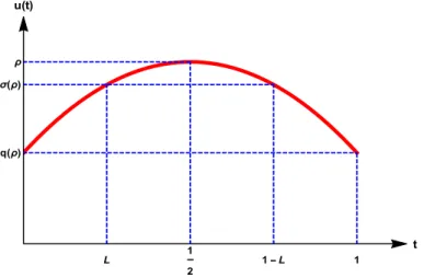
Letkuk∞ = ρ,u(L) =σ, andu(0) =u(1) =q, ˜F(s):=Rs
0 f˜(t)dtandF(s):=Rs
0 f(t)dt.
1 2
L 1-L 1
t q(ρ)
σ(ρ) ρ u(t)
Figure 1.5: Graph of a symmetric solutionuto (1.6).
Theorem 1.1. A symmetric solution (as in Figure 1.5) of (1.6) exists if and only if λ, ρ, σ and q satisfy:
√
λ= √1 2L
Z σ
q
dv q
F(q) + γ22q2 −F(v)
= √ 1 2(12−L)
Z ρ
σ
dv qF˜(ρ)−F˜(v)
,
F(q) + γ
2q2
2 −F(σ) =F˜(ρ)−F˜(σ).
In Section 2, we detail the proof of Theorem1.1. In Section 3, we provide biological implica- tions and numerical results.
2 Proof of Theorem 1.1
Supposeu>0 is a solution of (1.6). We first focus on the region(L,12). Multiply both sides of (1.6) byu0 and obtain
−(u0(x))2 2
0
=λF˜(u(x))0. Next, by integrating, we obtain
u0(x) = q
2λF˜(ρ)−F˜(u(x)); x∈L,12 , and further integration leads to
Z 1
2
x
u0(s) qF˜(ρ)−F˜(u(s))
ds=
Z 1
2
x
√
2λds; x∈ L,12 .
Now using the substitutionv=u(s)we obtain Z u(1
2) u(x)
1 qF˜(ρ)−F˜(v)
dv=√ 2λ
1 2−x
; x∈L,12 .
Settingx= Lwe have
Z ρ
σ
1 qF˜(ρ)−F˜(v)
dv=√ 2λ
1 2−L
. Further, solving forλwe obtain
λ=
√ 1
2(12−L)
Z ρ
σ
1 qF˜(ρ)−F˜(v)
dv
2
. (2.1)
We next focus on the region(0,L). Again by the above quadrature method, lettingu(0) = q, by the boundary conditions we get
u0(x) = s
2λ
F(q) + γ2q2
2 −F(u(x))
; x ∈[0,L]. Integrating on(0,x)we have
Z u(x) q
1 q
F(q) +γ22q2 −F(v)
dv=√
2λx; x ∈[0,L]. Hence substitutingx= Land solving forλyields
λ=
√1 2L
Z σ
q
1 q
F(q) + γ22q2 −F(v) dv
2
. (2.2)
Now usingu0(L−) =u0(L+), (2.1) and (2.2), we obtain:
√1 2L
Z σ
q
dv q
F(q) +γ22q2 −F(v)
= √ 1 2(12−L)
Z ρ
σ
dv qF˜(ρ)−F˜(v)
, (2.3)
F(q) + γ
2q2
2 −F(σ) =F˜(ρ)−F˜(σ). (2.4) In fact, givenρ,qandσsatisfy (2.3) and (2.4), we can back track and use the Implicit Function Theorem to obtain a solution as described in Figure1.5 with
λ=
√1 2L
Z σ
q
1 q
F(q) + γ22q2 −F(v) dv
2
. Hence the proof is complete.
We provide our computational results in the next section.
3 Computational results and biological implications
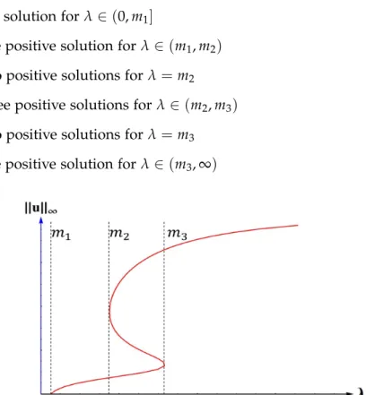
In [1], authors showed the occurrence of an S-shaped bifurcation curve for (1.2) for certain parameter ranges when grazing is confined to an interior region of (0, 1). Indeed, they nu- merically showed that for a fixedc=1.5, occurrence of an S-shaped bifurcation curve for (1.2) always happens ifKis chosen to be large enough. Namely, they showed that forK1 there existm1,m2, andm3such that (1.2) has (see Figure3.1):
• no positive solution forλ∈(0,m1]
• exactly one positive solution forλ∈(m1,m2)
• exactly two positive solutions forλ=m2
• exactly three positive solutions forλ∈(m2,m3)
• exactly two positive solutions forλ=m3
• exactly one positive solution forλ∈(m3,∞)
Figure 3.1: Occurrence of S-shaped bifurcation for (1.2).
We will obtain similar results when grazing is restricted to an interior patch, namely for (1.6). Moreover, we investigate the λ region where multiplicity of positive solutions occurs.
In particular, we fix all parameters with the exception of L and γ, where variations are im- plemented. First, we consider fixed values of L, namely L = 0.05, 0.30, and 0.45, and we demonstrate the evolution of the bifurcation diagrams for positive solutions when γ varies.
Next, forγ=50 (fixed), we demonstrate the evolution of the bifurcation diagrams for positive solutions when Lvaries.
We briefly explain how we obtain numerical bifurcation diagrams. Let γ > 0, L > 0, and M > 0 be fixed, and let xi = n+i1; i = 1, . . . ,n+1 for some n ≥ 1. Letting ρ = x1, we numerically solve the equations (2.3) and (2.4) simultaneously for σ and q using the FindRoot command in Mathematica. The values of σ andqare substituted into (2.2) to find the corresponding value ofλ. Repeating this procedure forρ= xi,i=2, . . . ,n+1, we obtain (λ,ρ)points for the bifurcation diagram.
Our research shows the following four cases:
1) For small values of L, multiplicity of positive solutions persists for certain ranges of λ irrespective of the value of hostility factor.
2) For large values of L, for no ranges of λ multiplicity occurs, regardless of the value of hostility factor.
3) For intermediate values of L, attainment or elimination of multiplicity regions is possible depending on the value of hostility factor.
4) For a fixed γ> 0, multiplicity regions persist for smallL and multiplicity regions are lost for largeL.
3.1 Bifurcation diagrams for fixed values of Lasγ varies
We closely examine our solutions via extracting the valueE(γ), where the non-trivial positive solution bifurcates from the trivial branch of solutions, as well as the interval(A(γ,L),B(γ,L)) corresponding to theλregion where multiplicity of positive solutions occurs.
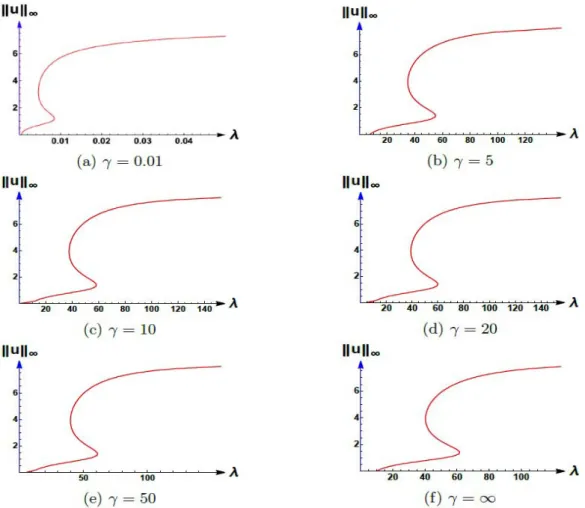
For L=0.05:
Figure 3.2: Bifurcation diagrams for (1.6) where K=10,c=1.5, andL=0.05.
γ E(γ) A(γ,L) B(γ,L) B(γ,L)−A(γ,L) 0.01 0.000411825 0.00459959 0.00848834 0.00388875
5 7.66329 34.9839 54.9993 20.0154
10 8.78401 37.6855 58.2939 20.6084
20 9.38331 39.0397 59.946 20.9063
50 9.75404 39.8512 60.937 21.0858
∞ 10.0055 40.3913 61.597 21.2057
Table 3.1: VaryingγwhileL=0.05.
Figure 3.3: Bifurcation diagrams for (1.6) whereK=10, c= 1.5, andL=0.30.
γ E(γ) A(γ,L) B(γ,L) B(γ,L)−A(γ,L) 5 7.63138 18.5239 19.2104 0.6865
20 9.35392 22.082 23.2109 1.1289 50 9.72529 22.8384 24.0726 1.2342
Table 3.2: Varying γwhileL=0.30.
Figure 3.4: Bifurcation diagrams for (1.6) whereK=10, c= 1.5, andL=0.45.
Remark 3.1. Our research concludes that whenK =10 andc=1.5 there existsL∗, L∗ ∈(0,12) with L∗ < L∗, such that when L < L∗ (grazing in a large subregion), the occurrence of multiple steady states for a range of λ persists for any hostility factor γ, and when L > L∗ (grazing in a small subregion), for any hostility factorγ, multiplicity of steady states does not occur for any λ. However, for L ∈ (L∗,L∗), there exists a γ∗(L)> 0 such that multiplicity of steady states for a range of λdoes occur for any hostility factorγ> γ∗(L).
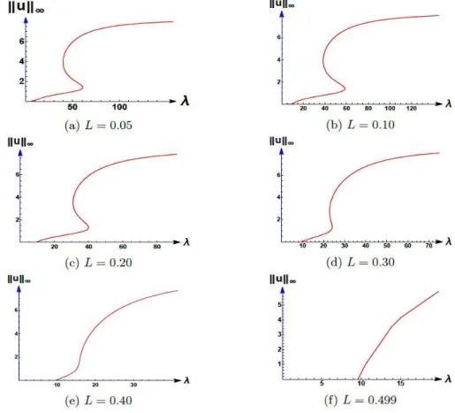
3.2 Bifurcation diagrams for a fixed value ofγ as Lvaries Forγ=50:
Figure 3.5: Bifurcation diagrams for (1.6) where K=10,c=1.5, andγ=50.
L E(γ) A(γ,L) B(γ,L) B(γ,L)−A(γ,L) 0.01 12.4772 40.0324 59.6438 19.6114
0.10 9.75354 38.3015 58.4055 20.104 0.20 9.74708 30.9087 40.1478 9.2391 0.30 9.72529 22.8384 24.0726 1.2342 Table 3.3: Varying Lwhileγ=50.
Remark 3.2. Note that for γ = 50, when K = 10 and c = 1.5 the occurrence of multiple positive steady states for a range ofλ is lost when Lis large (grazing in a small subregion). Furthermore, for any fixedγ> 0, occurrence of multiple positive steady states for a range of λare observed for L≈0 and occurrence of multiple positive steady states for anyλis lost for Llarge.
Acknowledgment
This material is based upon work supported by the National Science Foundation under Grant No. DMS-1516519.
References
[1] D. Butler, R. Shivaji, A. Tuck, S-shaped bifurcation curves for logistic growth and weak Allee effect growth models with grazing on an interior patch, in: Proceedings of the Ninth MSU-UAB Conference on Differential Equations and Computational Simulations, Electron. J.
Differ. Equ. Conf., Vol. 20, Texas State Univ., San Marcos, TX 2013, pp. 15–25.MR3128065 [2] J. T. Cronin, Movement and spatial population structure of a prairie planthopper,Ecol-
ogy 84(2003), No. 5, 1179–1188. https://doi.org/10.1890/0012-9658(2003)084[1179:
MASPSO]2.0.CO;2
[3] J. Cronin, J. Goddard, R. Shivaji, Effects of patch-matrix composition and indi- vidual movement response on population persistence at the patch-level, Bull. Math.
Biol. 81(2019), No. 10, 3933–3975. https://doi.org/10.1007/s11538-019-00634-9;
MR4012463
[4] N. Fonseka, J. Goddard, Q. Morris, R. Shivaji, B. Son, On the effects of the exterior ma- trix hostility and a U-shaped density dependent dispersal on a diffusive logistic growth model, Discrete Contin. Dyn. Syst. Ser. S, to appear. https://doi.org/10.3934/dcdss.
2020245
[5] N. Fonseka, R. Shivaji, B. Son, K. Spetzer, Classes of reaction diffusion equations where a parameter influences the equation as well as the boundary conditions, J. Math Anal. Appl. 476(2019), No. 2, 480–494. https://doi.org/10.1016/j.jmaa.2019.03.053;
MR3958013
[6] J. Goddard II, Q. Morris, C. Payne, R. Shivaji, A diffusive logistic equation with U- shaped density dependent dispersal on the boundary, Topol. Methods Nonlinear Anal.
53(2019), No. 1, 335–349.https://doi.org/10.12775/tmna.2018.047;MR3939159 [7] J. Goddard II, Q. Morris, S. Robinson, R. Shivaji, An exact bifurcation diagram for
a reaction diffusion equation arising in population dynamics, Bound. Value Probl. 2018, Paper No. 170, 17 pp.https://doi.org/10.1186/s13661-018-1090-z;MR3877704 [8] T. Laetsch, The number of solutions of a nonlinear two point boundary value problem,
Indiana Univ. Math. J. 20(1970), No. 1, 1–13. https://doi.org/10.1512/iumj.1970.20.
20001;MR269922
[9] R. M. May, Thresholds and breakpoints in ecosystems with a multiplicity of stable states, Nature269(1977), 471–477.https://doi.org/10.1038/269471a0
[10] F. J. Odendaal, P. Turchin, F. R. Stermitz, Influence of host-plant density and male harassment on the distribution of female Euphydryas anicia (Nymphalidae), Oecologia 78(1989), No. 2, 283–288.https://doi.org/10.1007/BF00377167
[11] A. M. Shapiro, The role of sexual behavior in density-related dispersal of pierid butter- flies,Am. Nat.104(1970), No. 938, 367–372.https://doi.org/10.1086/282670
[12] J. H. Steele, E. W. Henderson, Modeling long term fluctuations in fish stocks, Science 224(1984), 985–987.https://doi.org/10.1126/science.224.4652.985