DOI: 10.1556/606.2020.15.2.8 Vol. 15, No. 2, pp. 82–93 (2020) www.akademiai.com
LINEAR AND NONLINEAR DYNAMICAL ANALYSIS OF A CRANE MODEL
1 Hmoumen MAOURANE*, 2 Tamás SZABÓ
1,2 Robert Bosch Department of Mechatronics, Faculty of Mechanical Engineering and Informatics, University of Miskolc, Miskolc-Egyetemváros, H-3515, Hungary
e-mail: 1hhmoumen.maourane@gmail.com, 2szabo.tamas@uni-miskolc.hu Received 20 November 2019; accepted 8 January 2020
Abstract: This paper deals with the dynamical analysis of a crane model. Truss finite elements are used to discretize the suspending chains with the so called updated Lagrangian description. This nonlinear model is regarded to be the best approximation to which linear models are compared. The inertia and independent degrees of freedom are also taken into consideration by linear models. The goal is to find a linear model, which can be used as an observer in anti- sway control of a crane.
Keywords: Crane model, Nonlinear and linear dynamics, Finite element method
1. Introduction
Usually very simple mathematical pendulum models of the cranes are applied in papers [1]-[7]. The mass and its independent degree of freedom of the ropes/chains are neglected in these models. Though it is advantages to use a simple model as an observer in anti-sway control of cranes, but it may leads to inaccuracy in state space variables.
In this paper nonlinear and linear dynamical models of an overhead crane with chains will be formulated and analyzed. In addition to the payload, the inertia and independent Degree of Freedom (DoF) of the suspending chains are also considered.
Finite Element Method (FEM) is well applicable for the formulation of nonlinear and linear static and dynamic problems [8], [9]. The suspending chain perfectly flexible, i.e. it has no bending stiffness. The nonlinear model can be derived by the help of truss
* Corresponding Author
elements which can transfer only axial force [10] and perform 2D motions. The linear model practically is a taut string [11], which is discretized also with two node linear elements approximating only lateral motions. The solutions of the linear models are compared to the nonlinear counterpart.
2. Equations of motions of the crane models
The picture of a crane model is shown in Fig. 1. It is assumed that the displacements of the two parallel chains are the same therefore a single chain with double mass is a good substitution in a dynamical analysis. The chain is regarded as elastic, one dimensional structure, and can transmit only axial force along its x1 coordinate. The motion of the structure in plane (x, y) is investigated with nonlinear and linear approaches.
Fig. 1. Overhead lab crane model: 1. Trolley; 2. Chains; 3. Payload 2.1. Nonlinear model
In order to treat the nonlinear model of the overhead crane an incremental form of the principle of the virtual displacements with updated Lagrangian formulation [10] is used:
11 , 11
11 11 11 11
t V
t M t
V t
t V
t t t
V M
∆t t t M
∆t t V
t
dV e v
g M dV δ
dV dV
e e E δ
M dV δ
t t
t t
t
δ σ δ
ρ
η δ σ δ
ρ
∫
∫
∫
∫
∫
−
−
= +
+
+ +
+
u g
u u u
u&& &&
(1)
where ρt is the density of the material in the deformed configuration; t+∆t
u&& is a 2D
vector of the accelerations at time t+∆t; δu is the 2D vector of the virtual displacements; Vt is the volume of the structure at time t; M is the mass of the payload;
δuM is the 2D vector of the virtual displacements of mass M; g is the 2D vector of the gravity acceleration g; E is the Young’s modulus; e11t =du dx1 is the linear strain measured in axial direction in deformed configuration at time t; δe11 is the variation of the linear strain at the configuration time t; σ11t is the Cauchy stress of the one dimensional structure at time t; δη11is the variation of the quadratic portion of the nonlinear strain at the configuration time t. The quadratic portion of the nonlinear strain increment is written as
∂ + ∂
∂
= ∂
2 1 2 11 2 1
1
x v x
δ u η
δ , (2)
where u and v are the increments in displacements in axial x1 and its perpendicular direction, respectively. It is noted that (2) can be expressed also with global Cartesian displacement increments u, v
∂ + ∂
∂
= ∂
2 1 2 2 1
1
11 x
v x
δ u η
δ . (3)
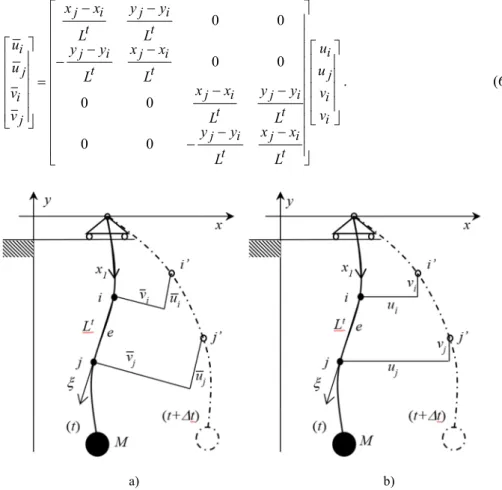
Truss elements are used to discretize (1). A truss element is a two node straight line member capable to transfer axial force only. Deformed length of the element is Lt, coordinate ξ measures the distance along the truss element, positive from node i to node j. The approximations for the axial displacement ue
( )
ξ and its perpendicular displacement ve( )
ξ along the element e are given as:( )
ji t t
e u
L u L
u ξ ξ
ξ +
−
= 1 , (4)
( )
ji t t
e v
L v L
v ξ ξ
ξ +
−
= 1 , (5)
where ui,ujand vi,vj are the increments in nodal displacements at element local coordinate system (see Fig. 2a). It is noted that dx1=dξ .
The local nodal displacement increments ui,ujand vi,vj can be related to the global Cartesian node displacement increments ui,uj and vi,vj(see Fig. 2b) via the following transformation:
−
− −
−
−
−
− −
−
−
=
i i j i
t i j t
i j
t i j t
i j t
i j t
i j
t i j t
i j
j i
j i
v v u u
L x x L
y
y L
y y L
x L x
x x L
y
y L
y y L
x x
v v u u
0 0
0 0
0 0
0 0
. (6)
a) b)
Fig. 2. Increments in nodal displacements of the nonlinear model given by a) local coordinates, b) global coordinates
It is also noted that the relation between the nodal forces in local and global coordinates are expressed similar way as (6), only the nodal displacements are replaced with nodal forces. The same transformation is also valid for the nodal accelerations.
The global Cartesian displacements in (3) and accelerations in (1) are approximated by the same linear interpolation functions as in (4) and (5):
( )
ji t t
e u
L u L
u ξ ξ +ξ
−
= 1 , (7)
( )
ji t t
e v
L v L
v ξ ξ
ξ +
−
= 1 , (8)
( )
t i t je
u
u L
u & & L ξ & & ξ & &
ξ +
−
= 1
, (9)( )
t i t je
v
v L
v & L & & & &
& ξ ξ
ξ +
−
= 1
, (10)where u&&i,
u & &
j, v&&i,v & &
j are nodal accelerations.The coordinates of the vector of displacement variationδuare approximated in the same way as the functions of (4), (5) and (7), (8).
Using (2)-(10) to determine the integrals in (1), it provides element mass matrix
=
2 0 1 0
0 2 0 1
1 0 2 0
0 1 0 2
6 t t t
e ρ A L
M , (11)
linear and geometric element stiffness matrices KLe and KGe on the left hand side of Eq. (1),
−
−
=
0 0 0 0
0 1 0 1
0 0 0 0
0 1 0 1 t t
Le L
E
K A ,
−
−
−
−
=
1 0 1 0
0 1 0 1
1 0 1 0
0 1 0 1 11 t t
Ge L
Aσ
K , (12)
the external and internal load vectors fGe, fσe in element local coordinate system on the right hand site of (1)
−
−
−
−
−
=
t i j
t i j
t i j
t i j
t t t Ge
L x x L
y y L
x x L
y y
L A g
2
f ρ ,
−
=
0 1 0 1 11
t e Atσ
fσ , (13)
where Atσ11t =Nt is the axial force of the truss element.
The element matrices are transformed to the global Cartesian coordinate system with the help of (6) then assembled according to the usual FEM process. The obtained equation of motion associated to (1) is written in matrix form as follows:
(
t)
gt t tG tL t
t q K K q f fσ
M+∆&&+ + ∆ = +∆ − , (14)
where Mt+∆t is the structural mass matrix; KtL and KtG are the structural linear and geometric stiffness matrices; fgt+∆t is the structural column vector of external loads;
σt
f is the structural column vector of internal loads; q&& is the structural column vector of nodal accelerations; ∆q is the structural column vector of the increments in nodal displacements. It is noted that the mass matrix is a constant matrix, i.e. is time invariant
t t+∆
=M
M , since the mass of the structure does not change in time.
The equation of motion (14) can be integrated numerically, e.g. by Newmark method. The steps of this method [10] are summarized as follows:
I. Initially the stiffness matrices KtL, KtG and the mass matrix
M
are formed and set the initial value of the displacements q0, the velocity q&0 and the accelerations q&&0.II. Form of the effective stiffness matrix at time t M
K K
K 2
ˆ 4
t t G t
L+ +∆
= . (15)
III. Form of the effective load vector fˆ at time t+∆t t
t t t
gt
tq q fσ M
f
f −
+
+ ∆
= +∆ 4 &
ˆ . (16)
IV. Solve the linear equation for the displacement increment ∆q
( )
0( )
ˆ, where 0.ˆ ∆qi =f i=
K (17)
V. Iteration for dynamic equilibrium (a) i=i+1
(b) Calculate
( )
i−1st approximation to accelerations, velocities, and displacements( )
t( )
i t tt
i t t
q q q
q&& & −&&
−∆
∆ ∆
= −
∆ +−
4 4
2 1
1 , (18)
( )
t( )
i t ti t q q
q& ∆ −&
= ∆ −
∆
+−1 1
4 , (19)
( )
t( )
i t ti q q
q +−∆1 =∆ −1 + . (20)
(c) Calculate
( )
i−1st effective out of balance load vector( ) ( )
t( )
i t tt i t gt t t
i
∆ +−
∆ +−
∆ +
∆
+−1 = − 1 − 1
ˆ f Mq fσ
f && . (21)
(d) Solve for the i’th correction to displacement increment
( )
i( )
ti+∆t=ˆ −1 ˆ∆qˆ f
K . (22)
(e) Calculate new displacement increments
( )
i q( )
i q( )
iq ∆ ∆ˆ
∆ = −1 + . (23)
(f) Iteration is terminated if
( ) ( )
t tol t
i
i ≤
∆ +
2 ˆ 2
∆ q
q
otherwise back to step (a). The
value of tolis prescribed by the user, its magnitude is10−6.
VI. If convergence ∆q=∆q
( )
i then accelerations, velocities, and displacements are determined as:t t t
t
t t
q q q
q& & &&
& −
−∆
=∆
∆
+ 4
4 ∆
2 , (24)
(
t t t)
t t
t+∆ =q + ∆t q +q +∆
q& 0.5 && && , (25)
q q
qt+∆t= t+∆ . (26)
Then increase the time with ∆t and jump to step II.
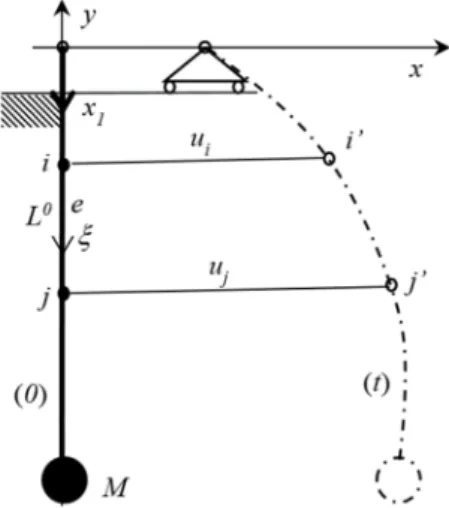
2.2. Linear crane model
Usually linear counterpart of the nonlinear equation of motion is needed in order to design a controller for a dynamical system. The crane model made of chain shown in Fig. 3 can be regarded as a taut string, which suffers relatively small lateral displacements. The axial force of the string due to gravity force is calculated in the rest position and assumed to be constant in the course its motion.
The linear equation (1D model) of motion of the crane can be derived by the help of the virtual displacements written for a taut string
t t V
t M t
V
R dV u u
u M dV u
u =
∫ +
∫ + 0 2 0
0 11
0 2
1
0 0
δ σ δ δ
ρ && &&
, (27)
where ρ0 is the density of the material at time zero; u&&t is the acceleration function in lateral direction; i.e. in horizontal direction at time t ; δu is the virtual lateral displacement function; V0 is the volume of the structure at time 0;
M
is the mass of the payload; u&&tMand δuM is the acceleration and virtual lateral displacements of mass M ; σ110 is the function of the axial stress due to gravity force determined in the rest position of the crane; and Rt is the virtual work of the external force obtained from displacement control.Fig. 3. Nodal displacements of the linear model
One dimensional linear line elements are used to discretize (27). The horizontal displacement is approximated along an element in local coordinate system:
( )
i je u
L u L
u 1 ξ0 ξ0
ξ +
−
= , (28)
where , are the horizontal nodal displacements of the element e.
The horizontal acceleration along an element is approximated also with the same interpolation functions
( )
i je u
L u L
u&& && &&
0
1 ξ0 ξ
ξ +
−
= , (29)
where u&&i,u&&j are horizontal nodal accelerations of the element e.
Substituting (28) and (29) into (27) the element mass matrix Me and stiffness matrix Ke can be derived
=
2 1
1 2 6
0 0 0A L
e ρ
M ,
=
1 1
1 1 0σ11 e A
K ,
= j e i
u q u ,
= j e i
u u
&
&
&
&
&
&
q , (30)
where qe is the element nodal displacement vector and q&&e is the element nodal acceleration vector, which are generated directly by the global Cartesian horizontal displacement approximation therefore no transformation is needed before assembling the structural matrices.
The linear equation of motion of the crane model is written as:
ft Kq q
M&&+ = , (31)
where M and K is the structural mass and stiffness matrices, ft is the column vector of the external forces due to displacement control, q is the structural vector of nodal displacements, q&& is the structural vector of nodal accelerations.
The linear differential equation (31) can be given also in state space form introducing new variables q=x1 and q& =x2:
u b Ax
x&= + , (32)
where
= 2 1 x
x x ,
= − − 0 K M
I
A 01 ,
= − − t
u M f
b 01
, and I is a unit matrix.
Numerical integration of (32) can be performed with number of standard methods, e.g. Runge-Kutta method or trapezoid rule, using Matlab or Scilab software system.
2.3. Numerical examples
Nonlinear and linear FEM programs have been developed using the above theory.
The length of the chains is 0.8 m, and it is subdivided into 10 uniform finite elements.
The linear version will be analyzed also with an FE mesh of two elements chain models.
The mass of the chain is 0.22 kg and two different payloads are exerted on the crane, the heavy one is 0.42 kg, the light one is 0.07 kg.
In order to compare their performances a simple crane motion will be simulated. In the beginning the trolley is moving with constant velocity v1=0.8ms along length
m 8 . 1=0
x , then it stops suddenly, thereafter the payload and the suspending chain will swing freely.
Motions of the cranes obtained for heavy payload using linear and nonlinear models are displayed in Fig. 4. It is clearly seen that the payload performs only horizontal motions in Fig. 4b. However the deformed shapes of the chains for both models are comparable in Fig. 4a and Fig. 4b.
a) b) Fig. 4. Position and shape of the chain during the motion
a) Nonlinear modeling b) Linear modeling
The computations have been performed for heavy and light payloads. The results are given in reference coordinate system and in relative coordinate system attached to the trolley, which are called in the sequel absolute and relative motions, respectively.
Absolute and relative motions of the payloads and the relative motions of the middle of the chain are shown in Fig. 5 - Fig. 7.
a) b)
Fig 5. a) Absolute motion of heavy payload; b) absolute motion of light payload
a) b)
Fig. 6. a) Relative motion of heavy payload; b) relative motion of the light payload
a) b)
Fig. 7. Relative motions of the middle point of the chain for a) heavy payload model;
b) light payload model
The displacements of nonlinear and linear models for heavy payload show good agreement in Fig. 5a and Fig. 6a, while the discrepancies are bigger for the light one in Fig. 5b and Fig. 6b.
It is clear from Fig. 7a and Fig. 7b that the chain vibration is significant. The discrepancies between the nonlinear and linear models are negligible for the heavy payload in the beginning (see Fig. 7a), then only relatively small shift can be detected later on. Except in the beginning the results of chain vibrations are less similar for light payload (see Fig. 7b). However during the controlling of the crane, the displacement of the payload is enforced to be close to the real motion of the crane. Therefore, a small shift in the solution is not a major problem.
4. Conclusion
The main goal of this investigation was to find linear models, which can be used as an observer in anti-sway control of the crane. Nonlinear and linear models have been used to simulate the motion of an overhead crane. The results confirmed the assumption that the vibration of the suspending chain is significant and advisable to take into consideration in linear models. The linear model with two finite elements provided also acceptable results compared to ten element mesh, therefore it is a good candidate to use as an observer.
Acknowledgements
The described article was carried out as part of the EFOP-3.6.1-16-2016-00011
‘Younger and Renewing University - Innovative Knowledge City - institutional development of the University of Miskolc aiming at intelligent specialization’ project implemented in the framework of the Szechenyi 2020 program. The realization of this project is supported by the European Union, co-financed by the European Social Fund.
Open Access statement
This is an open-access article distributed under the terms of the Creative Commons Attribution 4.0 International License (https://creativecommons.org/licenses/by/4.0/), which permits unrestricted use, distribution, and reproduction in any medium, provided the original author and source are credited, a link to the CC License is provided, and changes - if any - are indicated. (SID_1)
References
[1] Wahyudi, Jalani J., Muhida R., Salami M. J. E. Control strategy for automatic Gantry Crane systems: A practical and intelligent approach, International Journal of Advanced Robotic Systems, Vol. 4, No. 4, 2007, pp. 447‒456.
[2] Won I. S., Hoang N. Q., Lee S. G., Ryu J. K. Comparative study of energy-based control design for overhead cranes, International Robotics and Automation Journal, Vol. 4, No. 3, 2018, pp. 197‒203.
[3] Kaur A., Priyahansha, Kumari S., Singh T. Position control of overhead cranes using fuzzy controller, International Journal of Advanced Research in Electrical, Electronics and Instrumentation Engineering, Vol. 3, No. 5, 2014, pp. 9341‒9350.
[4] Almutairi N. B., Zribi M. Fuzzy controllers for a Gantry Crane system with experimental verifications, Mathematical Problems in Engineering, Vol. 2016, Paper No. 1965923, pages 1‒17.
[5] Ahmad M. A. Active Sway suppression techniques of a Gantry Crane system, European Journal of Scientific Research, Vol. 27, No. 3, 2009, pp. 322‒333.
[6] Ospina-Henao P. A., L´opez-Suspes F. Dynamic analysis and control PID path of a model type gantry crane, Journal of Physics, Conf. Series, Vol. 850, 2017, pages 1‒14.
[7] Kharola1 A., Patil P. Mathematical modeling and performance comparison of overhead cranes using soft-computing techniques, International Journal of Mechatronics, Electrical and Computer Technology, Vol. 7, No. 23, 2017, pp. 3188‒3200.
[8] Vătăman A., Ciutina A., Grecea D. Numerical analysis of short link steel eccentrically braced frames under seismic action, Pollack Periodica, Vol. 11, No. 2, 2016, pp. 29‒42.
[9] Hajdu F., Szalai P., Mika P., Kuti R. Parameter identification of a fire truck suspension for vibration analysis, Pollack Periodica, Vol. 14, No. 3, 2019, pp. 51‒62.
[10] Bathe K. J. Finite element procedures, Prentice Hall, Pearson Education Inc, 2006.
[11] Meirovich L. Fundamentals of vibrations, McGraw-Hill, New York, 2001.