El e c t ro nic J
o f
Pr
ob a bi l i t y
Electron. J. Probab.26(2021), article no. 99, 1–18.
ISSN:1083-6489 https://doi.org/10.1214/21-EJP665
Invariant embeddings of unimodular random planar graphs
*Itai Benjamini
†and Ádám Timár
‡Abstract
Consider an ergodic unimodular random one-ended planar graphGof finite expected degree. We prove that it has an isometry-invariant locally finite embedding in the Euclidean plane if and only if it is invariantly amenable. By “locally finite” we mean that any bounded open set intersects finitely many embedded edges. In particular, there exist invariant embeddings in the Euclidean plane for the Uniform Infinite Planar Triangulation and for the critical Augmented Galton-Watson Tree conditioned to survive. Roughly speaking, a unimodular embedding ofG is one that is jointly unimodular withGwhen viewed as a decoration. We show thatGhas a unimodular embedding in the hyperbolic plane if it is invariantly nonamenable, and it has a unimodular embedding in the Euclidean plane if and only if it is invariantly amenable.
Similar claims hold for representations by tilings instead of embeddings.
Keywords:random planar graphs; invariant embedding; unimodular embedding.
MSC2020 subject classifications:Primary 60D05, Secondary 60K99.
Submitted to EJP on April 8, 2021, final version accepted on June 7, 2021.
1 Introduction
1.1 Main results
Homogeneous (say, vertex-transitive) tilings of the Euclidean and hyperbolic planes are well-understood classical objects. Here we studyrandomplanar tilings that are
“homogeneous” in some sense: they have an isometry-invariant law or satisfy a certain stationarity property, called unimodularity (see the definitions below). We are asking the question: when does a random infinite graph that is known to be almost surely planar have such a “homogeneous” embedding into the Euclidean or hyperbolic plane without accumulation points (i.e., alocally finiteembedding)?
*The second author was supported by the ERC Consolidator Grant 772466 “NOISE” and by Icelandic Research Fund Grant 185233-051.
†Weizmann Institute of Science, Israel. E-mail:itai.benjamini@weizmann.ac.il
‡University of Iceland, Iceland and Alfréd Rényi Institute of Mathematics, Hungary.
E-mail:madaramit@gmail.com
After formalizing the above question, one finds right away that a necessary condition is that the random graph with a properly chosen root is unimodular itself, so from now on, we are only interested in this family of random rooted graphs. Unimodularity, embedding and representation by a tiling will be defined later in the introduction. We say that the random rooted graph(G, o)hasfinite expected degree if the expected degree ofo is finite.
Theorem 1.1.An ergodic unimodular random one-ended planar graphGof finite ex- pected degree has an isometry-invariant locally finite embedding into the Euclidean plane if and only ifG is invariantly amenable. The same condition is necessary and sufficient to representGby an isometry-invariant locally finite tiling.
One source of interest in invariant random embeddings of unimodular random graphs is examples such as the Uniform Infinite Planar Triangulation (UIPT). Theorem 1.1 applies for the UIPT, as stated in Corollary 4.3.
WhenGhas an embedding into the Euclidean or hyperbolic plane, the relative location of the embedded vertices and edges by this embedding from the viewpoint of each vertex can be used to decorate the vertices. If the decorated graph is still unimodular, we call the embedding unimodular. The more precise definition is given in the next subsection.
Theorem 1.2.An ergodic unimodular random one-ended planar graphGof finite ex- pected degree has a unimodular locally finite embedding
• into the Euclidean plane if and only ifGis invariantly amenable,
• into the hyperbolic plane ifGis invariantly nonamenable.
One can construct the embedding so that every edge is mapped into a broken line segment (piece-wise geodesic curve). We mention that here and in the next theorem, the
“only if” part is missing from the second claim because of examples such as Example 1.6.
With some extra condition this could be ruled out and have a full characterization in the theorems; see the discussion after the example.
Theorem 1.3.An ergodic unimodular random one-ended planar graphGof finite ex- pected degree can be represented by a unimodular locally finite tiling
• in the Euclidean plane if and only ifGis invariantly amenable,
• in the hyperbolic plane ifGis invariantly nonamenable.
The tilings guaranteed by the theorem are such that the expected area of the tile containing the origin is finite. Similarly to embeddings, we say that a tiling is locally finite if every bounded open subset of the plane intersects finitely many tiles. We will give precise definitions later in this section. We mention that the tiles in the above theorem can be required to be bounded polygons.
Theorems 1.2 and 1.3 provide essentially complete dichotomic descriptions for the one-ended case. The cases not covered are those ofGwith 2 or infinitely many ends, in which situation a graph may or may not have any invariant embedding into one of the Euclidean or the hyperbolic plane (Remark 1.5). We do not treat 2 or infinitely many ends here, to avoid technical distractions from our main point.
In the case of invariantly amenable graphs, we will first construct an invariant embedding into the Euclidean plane, starting from a suitable invariant point process as the vertex set. This invariant embedded graph automatically defines a unimodular embedding. On the other hand, for invariantly nonamenable graphs, a unimodular embedding into the hyperbolic plane will be constructed directly, via circle packings.
(This circle packing embedding would not work in the Euclidean case, because Euclidean scalings provide an extra non-compact degree of freedom, making it unclear how to achieve unimodularity.) The intuitive claim that such a unimodular embedding is the
“Palm version” of an invariant embedding does not seem to have been established in the hyperbolic setup; a similar statement in the Euclidean case is in the focus of [18].
This is the reason for the asymmetry in the Euclidean and hyperbolic cases of the above theorems. A new preprint by the second author and László Tóth [38] settles the question of invariant embedding of nonamenable graphs into the hyperbolic plane, together with the cases of 2 and infinitely many ended graphs, left open by the present paper.
1.2 Definitions
Our focus is on Euclidean and hyperbolic spaces, hence the definitions will be phrased in this setting. One could ask questions in greater generality, for example by taking Lie groups as underlying spaces.
Without loss of generalityfrom now on we assume thatGis a simple graph, that is, it has no loop-edges or parallel edges. We also assume thatall the degrees are finiteinG. We will define two types of invariance property that a random graph embedded in some space may have: one is from the viewpoint of a root in the graph (unimodular embedding), and the other is with respect to the isometries of the enveloping space (isometry-invariant embedding). Before going into the formal definitions, let us show two examples that emphasize the difference between the two notions. Consider a (deterministic) embedding ofZas a biinfinite straight line inR2subdivided by vertices such that two adjacent vertices have distance 1. If we fix an arbitrary vertex of this embedded graph, the scenery seen around this vertex remains the same (trivially) if we randomly reroot it to a neighbor. However, if we view the embedded graph from a point of the underlying space there is no similar invariance: applying an isomorphism that does not fix the embedded path will change what we see. So in this example the distribution (which is an atomic measure here) is invariant fromt he viewpoint of the embedded graph, but not from the viewpoint of the enveloping space. On the other hand, considerZ2, and for every vertex(i, j)∈Z2, ask= 2,3, . . ., add a new vertex(i+ 2−1− 2−k, j+ 2−1−2−k)and a new straight-line-edge between(i+ 2−1−2−k, j+ 2−1−2−k) and(i+ 2−1−2−k+1, j+ 2−1−2−k+1). After taking a random isometry ofR2uniformly from those mapping 0 to some element of[0,1)2, and applying it to our embedded graph, we get an isometry-invariant embedded graph. However, it is not possible to assign a root to this graph in a way that will make it unimodular (“rerooting-invariant”), because the graph itself is not unimodular, having isolated ends. Let us highlight that in this last example the vertex set has infinite intensity, which possibility we will rule out and only allow finite intensity embeddings in the definition. Nevertheless, the example may shed some light on the difference between the two close notions of invariance in our scope.
Next we give a precise definition of unimodularity. First we are using random walks, as this seems to be more natural to describe when unimodular random embeddings are considered. LetG∗be the collection of all locally finite connected rooted graphs up to rooted isomorphism, and letG∗∗be the collection of all locally finite connected graphs with a distinguished ordered pair of vertices up to isomorphism preserving this ordered pair. We often refer to an element ofG∗as arooted graph(G, o), without explicitly saying that we mean the equivalence class that it represents inG∗. Let(G, o)be a random rooted graph and suppose thatohas finite expected degree. Reweight the distribution of(G, o) by the Radon-Nikodym derivativedeg(o)/E(deg(o)). We will refer to such a reweighting by saying that webias by the degree of the root. Denote the new random graph by(G0, o0). LetX0 =o0 and letX1be a uniformly chosen neighbor ofX0. We say thatG= (G, o)is unimodular if(G0, X0, X1)has the same distribution as(G0, X1, X0). See [1] or [6] for the proof that this is equivalent to the original definition of unimodularity for graphs in [1], which we recall in the next paragraph. One may consider some decoration or marking on rooted graphs, and extend the above definition in the obvious way. Whenever there
is a decoration, given as a functionf onV(G)or as a subgraphU ≤G, we denote this decorated rooted graph by(G, o;f),(G, o;U). In case of several decorations, we can list them all after the semicolon.
The original definition of unimodularity, equivalent to the previous one, is the fol- lowing. Consider an arbitrary Borel functionf :G∗∗ →R+0. Then it has to satisfy the following equation
Z X
y∈V(G)
f(G, x, y)dµ((G, x)) =
Z X
y∈V(G)
f(G, y, x)dµ((G, x)). (1.1)
Here we do not distinguish between(G, x)as a rooted graph and as a representative of its equivalence class in G∗∗. This is standard in the literature and will not cause ambiguity. Equation (1.1) is usually referred to as the “Mass Transport Principle” (MTP).
This equivalent definition of unimodularity naturally extends to decorated rooted graphs, one just has to consider Borel functionsf from the suitable space.
LetM be some homogeneous metric space with some point0fixed; for our purpose we can just assume that it is a Euclidean or hyperbolic space. LetIsom(M)be the group of isometries ofM. For a graphG, anembeddingιofGinto a Euclidean or hyperbolic spaceM is a map fromV(G)∪E(G)that maps injectively every point inV(G)to a point ofM, and every edge{x, y} to (the image of) a simple curve inM between ι(x)and ι(y), in a way that two such images can intersect only in endpoints that they share. The embeddings that we consider are locally finite (i.e., every compact set is intersected by finitely many embedded edges or vertices), henceM\ι(V(G)∪E(G))is open. The connected components ofM\ι(V(G)∪E(G))are calledfaces.
Let(G, o)be some unimodular random graph. For almost everyG, letιG=ιbe some embedding ofGintoM. We can encode the embedding by a labelling of the vertices coming from a suitable mark space that tells us what the embedding is for every ball up to orientation-preserving isometries ofM. (See [5] for more detailed examples of such labellings.) From this labelling, one can reconstructιup toIsom(M). We say that ιis aunimodular embedding ofGtoM, if the labelling is a unimodular decoration of G. We emphasize again that aιand anyι0 =γ◦ι(γ ∈Isom(M)) give rise to the same unimodular embedding.
A unimodular random graph (G, o) is invariantly amenable (or just amenable) if for every > 0 there is a random subset U ⊂V(G)such that (G, o;U)is unimodular, every component of G\U is finite, andP(o ∈ U) < . (In [1] this property is called hyperfiniteness, and is shown to be equivalent to their definition of invariant amenability in Theorem 8.5 wheneverGhas finite expected degree – an assumption that we will always make.) If this property fails to hold, thenGisinvariantly nonamenable(or just nonamenable). In the rest of this paper we will drop “invariantly” and simply call unimodular random graphs amenable or nonamenable, but the reader should keep in mind that these terms are different from the ones used for a deterministic graph. For the relationship of this notion of amenability to almost sure amenability or anchored amenability, see the discussion in [1] after the definition, and Theorem 8.5 therein for some equivalents.
Consider a random graphDdrawn inM in a measurable way, with a distribution that is invariant under Isom(M). Call such aD invariant. The setV ⊂ M of drawn vertices ofDforms an invariant point process inM. Say that theintensityofDis the expected number of points ofV in a ball with unit volume. (This expectation does not depend on the location of the unit box, because of invariance.) Suppose thatDhas finite intensity, and consider thePalm versionD∗ ofD. By this we meanDconditioned on 0∈ V. By standard theory of point processes and the assumption on finite intensity, this definition makes sense andD∗is a random graph drawn inM with a vertex in0. Now let
(G, o)be a unimodular random graph. By aninvariant embedding(orisometry-invariant embedding) ofGintoM we mean a random graphDdrawn inM of isometry-invariant ditribution that has finite intensity, and with the property that(D∗,0)viewed only as an element ofG∗has the same distribution as(G, o). (The fact that(D∗,0)is unimodular has been well-known, see Example 9.5 in [1].)
Remark 1.4.The term “unimodular embedding” was first used in [3], and the definition there is equivalent to ours. Similar notions existed earlier in the point process literature.
A unimodular embedding tells the location of all embedded edges and vertices from the viewpoint of the root vertex. Specifically, the embedded vertices can be thought of as a point process with a point in the origin, and up to equivalence by isometries fixing the origin. The notion ofpoint-stationarity, introduced by Thorisson [32] for processes with a point at the origin, requires an invariance under rerooting, similarly to the random walk definition for unimodularity. In fact, the definition of point-stationarity for point processes applies to embedded graphs right away, and the existence of a unimodular embedding is equivalent to the existence of a point-stationary graph whose underlying graph has the same distribution as the given graph. Our observation (from [1]) that the Palm version of an isometry-invariant embedding is unimodular has been essentially known since Mecke [28], whose intrinsic characterization shows that the Palm version of a (translation-)invariant point process is always point-stationary.
We will denote the Euclidean plane by R2, and the hyperbolic plane by H2. Note that an invariant embedding of a unimodular graph automatically has finite intensity, since it was required for the definition to make sense. We are interested in embeddings where in addition, no bounded open set is intersected by infinitely many embedded edges, that is,locally finite embeddings. The notion of local finiteness is invariant under isometries, so one can define it for unimodular embeddings as well. By atilingwe mean a collection of pairwise disjoint connected polygons (“tiles”) such that the union of their closures isM. We will be interested in tilings where every compact subset ofM is intersected by only finitely many types. A tiling defines a graph where the tiles are the vertices and two of them are adjacent if they share some nontrivial line segment on their boundary. The definition of invariant tilings that represent(G, o)is similar to that of invariant embeddings. Namely, suppose that a random tiling is isometry-invariant and the tile of the origin has finite area almost surely. Take a uniform random point in every tile and consider the Palm version of this point process together with the tiles on it. If the rooted graph defined by this tiling (rooted at the tile of the origin) has the same distribution as(G, o)then we say that the invariant tiling represents(G, o).
Remark 1.5.It is well-known that an infinite unimodular random graph can have only 1, 2 or infinitely many ends, [1]. As mentioned earlier, Theorems 1.2 and 1.3 do not cover the case of 2 ends and infinitely many ends. If a unimodular random planar graphGhas infinitely many ends almost surely, then it is nonamenable. There are examples where a unimodular embedding intoH2is possible, and examples when it is not (and similarly for invariant embeddings and for tilings). For the latter, letGbe the free product of the edge graph of a transitive hyperbolic tiling and a single edge, andGbe supported in this single transitive graph. It is easy to check that any planar embedding of this graph is such that the embedded vertices have infinitely many accumulation points. Hence there is no locally finite invariant embedding or unimodular embedding for this graph. On the other hand, the 3-regular treeT3does have an invariant embedding intoH2, which simply gives rise to a unimodular embedding. To see such an invariant embedding, take the Ford horocyclic tiling (see, e.g., Figure 3.3 in [27]), letF be a fundamental domain that contains the origin, and choose a random isometry that maps the origin to a point of F according to Haar measure. Consider the centers of the interstices (bounded pieces
in the complement of the disks) and the straight lines between neighboring ones (which will all have the same length), and apply the random isometry to this embedded graph of T3.
The next example shows that “zero intensity” is possible in case of unimodular embeddings.
Example 1.6.Consider Gto be Z almost surely, and letM be the hyperbolic plane.
Take an infinite geodesicγinM, fix a point0 ∈γ, and letg be an isometry ofM that preservesγand maps0to someg(0)6= 0. Consider the embedded graph with vertex set {gi(0), i∈Z}and embedded edges being the pieces ofγbetween pairsgi(0)andgi+1(0). One can check that this way we defined a unimodular embedding ofZintoM. However, it is not possible to embedZ(or any amenable graph) intoM in an isometry-invariant way.
One could define intensity for unimodular embeddings. We will not need this, but it could be defined as the reciprocal of the unique numberrthat ensures that the stable allocation on the embedded vertices with cell-volume-limitris a full allocation (with r=∞standing for zero intensity); see [21] for the definition. Forbiding zero intensity, one could rule out pathologies as Example 1.6. Then Theorems 1.2 and 1.3 would become full characterizations (by a suitable modification of the proofs in Section 5 for the added
“only if” parts).
Acyclic permutationofnelements is a permutation that consists of a single cycle of lengthn. A combinatorial embeddingof a planar graphGis a collection of cyclic permutationsπv of the edges incident to v overv ∈ V(G), and such that there is an embedding ofGin the plane where the clockwise order of the edges on every vertexv isπv for everyv ∈V(G). A combinatorial embedding is unimodular if the decoration {πv}is a unimodular decoration. The notion of unimodular combinatorial embeddings (and maps) was implicitly introduced in Example 9.6 of [1]. Note that this definition does not use any underlying metric on the plane, as it defines an embedding only up to homeomorphisms. For a given edgee, choose an orientation ofewithe− being the tail ande+the head. Consider the edgeπe−(e)oriented such thate− is its head. Repeat this procedure for this new oriented edge, and iterate until we arrive back to(e−, e+). Call the resulting sequence of edges afaceof the combinatorial embedding. One can check that the faces of actual embeddings coincide with the bounded domains surrounded by the respective faces of the corresponding combinatorial embedding. In [36] it is shown that being unimodular and planar guarantees the existence of a unimodular combinatorial embedding in general, see Theorem 2.1.
Remark 1.7.The existence of a unimodular combinatorial embedding does not automat- ically provide us with a unimodular embedding intoR2orH2, but the other direction is obvious. To summarize: an isometry-invariant embedding defines a unimodular em- bedding (as verified in the proof of Theorem 1.2), and a unimodular embedding trivially defines a unimodular combinatorial embedding. None of the other directions holds a priori.
For a given graphG, acircle packingrepresentation ofGis a collection of circles in the plane such that the circles are in bijection withV(G)and two circles are tangent if and only if the corresponding vertices are adjacent inG. Thenerveof a circle packing is the graph that it represents. For a given circle packingP inR2, consider the union of all the disks inP and their boundaries and its further union with all the bounded connected pieces (interstices) bounded by finitely many circles inP. Call the resulting set thecarrierofP.
Theorem 1.8.(He-Schramm, [16], [17], Schramm, [31])LetGbe a one-ended infinite planar triangulated graph. ThenGeither has a circle packing representation whose
carrier is the plane or it has a circle packing representation whose carrier is the unit disk, but not both.
• In the former case (whenGis parabolic), the representation in the plane is unique up to isometries and dilations.
• In the latter case (whenGis hyperbolic), the representation in the unit disk is unique up to Möbius transformations and reflections fixing the disk.
In the first case they called the graphCP parabolic, while in the second case they called itCP hyperbolic. They found several characterizing properties for this duality, such as the recurrence/transience of simple random walk. Earlier, Schramm [31] proved the uniqueness of these circle packings up to some transformations. See also [29].
1.3 Connections to past research
Our topic is at the meeting point of isometry-invariant point processes and unimodular random graphs. The former has been a widely studied subject for many decades (see, e.g., the monographs [32], [25]), mostly in the setup of stationary (translation-invariant) point processes in Euclidean spaces. A key problem in the present work is to represent certain graphs on the configuration points of a point process, in a covariant and measurable way.
Questions of this flavor have been extensively studied for particular classes of graphs in the past, such as one-ended trees, biinfinite paths ([12], [20], [34]) or perfect matchings (see, e.g., [22], [19]). Note however, that while in these settings only graphs on the vertex set have to be defined, in our context we also need toembed the edgesinto the underlying space.
Unimodular random graphs were first defined in [1], but similar ideas existed earlier (see references in [1]). They have attracted a lot of attention because of their connection to approximability by finite graphs (see [30] for the importance of such approximability in group theory), because of closely related notions in other areas (such as graphings in measurable group theory, see, e.g., [26]), and for being a natural generalization of group-invariant percolation. One can think of the notion of unimodular random graphs as a generalization of “percolation on a transitive graph with a unimodular group of automorphism, viewed from a fixed vertex”, which makes it analogous to the Palm version of a point process. The direct connection is that invariant point processes as well as unimodular random graphs satisfy the Mass Transport Principle. That the Palm version of a random graph invariantly drawn in the plane is always unimodular as a planar graph was already proved by Aldous and Lyons [1] (see also our Remark 1.4), and our main results can be regarded as the converse to this claim.
A study of unimodular random planar graphs was initiated by Angel, Hutchcroft, Nachmias and Ray in [2] for the class of triangulations, and they showed that for a locally finite ergodic unimodular triangulated planar simple graph, being CP parabolic is equivalent to invariant amenability. In [3], unimodular planar graphs were further studied, without the assumption of being triangulated, but with the assumption that the unimodular graph comes together with a unimodular combinatorial embedding, in which case this joint object is called aunimodular planar map. Several criteria were identified as equivalents to invariant amenability. Theorems 1.2 and 1.3 can be thought of as further examples of the dichotomy.
As an example, consider the Uniform Infinite Planar Triangulation (UIPT), first defined by Angel and Schramm in [4]. The UIPT is a random graph that is unimodular (because it arises as the local limit of finite graphs) and planar (because all these finite graphs are planar), and moreover, the graph comes together with a unimodular combinatorial embedding (inherited from the finite graphs). Nevertheless, a combinatorial embedding defines an actual embedding into the plane only up to homeomorphisms. Now, if we are
given not only the topology but also some homogeneous metric on the plane (and the the only homogeneous simply connected Riemannian manifolds of infinite volume, up to scaling, are the Euclidean and the hyperbolic planes, see Theorem 3.8.2 in [33]), then it is natural to require the unimodular embedding to exist not just up to homeomorphisms but up to isometries. This latter, a unimodular embedding up to isometries, is what we defined simply as a unimodular embedding. If a unimodular embedding exists, one can further ask whether an isometry-invariant embedding exists with this given unimodular embedding. This last question takes us back to the theory of point processes, where analogous questions were addressed: is a unimodular point process of positive intensity (that is, a point process satisfying a MTP, with a point in the origin, whose Voronoi cell has finite expected volume) always the Palm version of a isometry/translation-invariant point process? This question was settled by Heveling and Last [18] in the positive (who use the term point-shift stationary for what we called here a unimodular point process) for translation invariant processes.
Here we are interested in planar graphs, but it is reasonable to ask what happens in higher dimensions. In [35] it is shown (in the dual language of tilings) that every one-ended amenable unimodular transitive graph has an isometry-invariant embedding intoRdwhend≥3. The proof generalizes from transitive to random unimodular graphs.
2 Unimodular planar triangulation of unimodular planar graphs
The following theorem was proved in [36].
Theorem 2.1.([36])Let(G, o)be a unimodular random planar graph of finite expected degree. Then(G, o)has a unimodular combinatorial embedding into the plane.
Recall that having a unimodular combinatorial embedding is a weaker requirement than having a unimodular or an invariant embedding, see Remark 1.7.
Theorem 2.2.Let(G, o)be a unimodular planar graph of finite expected degree. Then there is a unimodular decorated graph(G+, o+, S)whereSis a connected subgraph ofG+ and such that(S, o+)conditioned ono+∈Shas the same distribution as(G, o). andG+is a planar triangulation of finite expected degree. IfGis simple thenG+is also simple. IfG has one end thenG+has one end.
Proof. By Theorem 2.1,Ghas a unimodular combinatorial embedding into the plane. Fix such an embedding. The collection of faces is also jointly unimodular withG.
LetF be an unbounded face. By exploring the vertices ofF along the boundary, a function fromZto the boundary is obtained which is not necessarily injective. Fix such a function, chooseξ∈ {0,1}uniformly at random, and for every pair{2k+ξ,2k+ξ+ 1}
(k∈Z), add a new vertexvkto the graph, and connect it to2k+ξ,2k+ξ−1and2k+ξ+ 1. Finally, add an edge betweenvk andvk+1 for everyk∈ Z. Now, in the resulting new graph we have a new infinite face, whose boundary is the biinfinite path induced by . . . , v−1, v0, v1, . . .. Repeat the previous procedure for this biinfinite path, and so on, ad infinitum.
For every bounded faceF do the following. IfF hasnedges on its boundary, then add a new cycleCof length[(n+ 1)/2]inside this face. Add edges that connect these new vertices to the boundary vertices ofF so that planarity is not violated, in such a way that we connect every vertex ofCto the vertices of two consecutive edges ofF, except maybe one vertex ofCwhich is connected to one edge ofF. Then for every vertexxof F and two consecutive edges ofF containingx, there are at most two new edges added toxbetween these two consecutive edges. Hence the degree ofxis at most trippled by the end of this procedure. Repeat this step for the new face, surrounded byC, as long
as|C| ≥6. Otherwise just add a new vertex and connect it to every vertex ofC. In each step, if there is more than one option, choose one of the options randomly and uniformly.
When doing this for everyF, in the limit we get a triangulationG+. All the operations preserved planarity, henceG+ is planar. One can define a functionτ : V(G+) →V(G) (possibly using extra randomness) such that E|τ−1(o)| < ∞. Therefore, by similar arguments to Example 9.8 of [1] (see Subsection 1.4 in [8] for more details), G+ is unimodular with the random rooto+chosen as follows: we first bias(G, o)by weights proportional to|τ−1(o)|, and theno+can be sampled by choosing a uniform element of τ−1(o).
From the same argument in [8] it follows that the expected degree ofo+ is bounded bymax{3D,7}, whereD is an upper bound on the expected degree of the root in(G, o). Here we are using the fact that the vertices inV(G)have received at most twice as many new edges as their degree inG(at most two new edges between each pair of consecutive edges on a face), and every new vertex has at most 7 incident edges.
Before proceeding, let us state some consequences of Theorem 2.1 related to percola- tion, as the methods of [7] become available for the planar graph that have a unimodular combinatorial embedding. This corollary was unnoticed in [36], the source of Theorem 2.1, so we present it here. Call a planar graphGedge-maximal, if for anyx, y∈V(G), such that{x, y} 6∈E(G)andx6=y,G∪ {{x, y}}is nonplanar. Edge maximality means that any planar embedding ofGis triangulated.
Corollary 2.3.LetGbe an ergodic nonamenable unimodular random planar graph with finite expected degree and one end, and consider Bernoulli(p) bond or site percolation.
Then there existpc andpu > pc such that there is no infinite component whenever p∈[0, pc], there are infinitely many infinite components forp∈(pc, pu), and there is a unique infinite component forp∈[pu,1]. IfGis edge-maximal and we percolate on the vertices, thenpc<1/2.
Proof. The claim that there is no infinite component inpc is known to be true for any nonamenable graph, see Theorem 8.11 in [1]. Thatpc< puand there is uniqueness inpu
are proved for graphs where a unimodular planar combinatorial embedding is given in Theorem 8.12 in [1] (based on [7]); combined with Theorem 2.1 (a result from [36]) they show the claims here. Finally, for the claim aboutpc<1/2, the proof of Theorem 6.2 in [7] extends, once we have a unimodular combinatorial embedding as in Theorem 2.1.
A bound pc < 1/2 is proved in [15] for general graphs with a minimum degree requirement.
3 Invariant circle packing representations of nonamenable graphs
The next theorem is a simple consequence of results by He and Schramm.
Theorem 3.1.Suppose thatG= (G, o)is a one-ended nonamenable ergodic unimodular random planar simple graph with finite expected degree. ThenGcan be represented by a unimodular circle packing in the hyperbolic plane. Consequently,Ghas a unimodular embedding into the hyperbolic planeH, andGcan be represented by an invariant tiling.
Proof of Theorem 3.1. We may assume that G is triangulated. Otherwise apply first the proof for the triangulated supergraphG+ in Theorem 2.2, and then only keep the circles that represent vertices inV(G). We know from Theorem 1.8 thatGhas a unique representation in the hyperbolic plane up to hyperbolic isometries. From the proof by He and Schramm it follows, as explained in detail in Subsection 3.4.1 of [2], that
the hyperbolic radius of the circle representing vertexv is a measurable function of (G, v)∈ G∗. Hence the circle packing (Gas a graph marked with the unique circle packing, where the marks are telling the embedding of the vertices together with an extra label representing the radius) is unimodular.
One can turn the circle packing into a tiling of the same adjacency structure by properly subdividing every component of the complement of the disks into finite pieces and attaching them to suitably chosen neighboring disks. We omit the details.
4 Invariant embeddings of amenable unimodular planar graphs
In this section we will prove the amenable part of Theorem 1.1. We will later use this invariant embedding to constuct a unimodular embedding and prove the amenable parts of Theorems 1.2 and 1.3. One may wonder if a unimodular embedding could be found directly, following the lines of the proof for the hyperbolic case, but a key part which does not go through is the following. The uniqueness in the He-Schramm Theorem 1.8 is up to isometries in the nonamenable (hyperbolic) case, and hence it could be used in the construction of the unimodular embedding, which is also defined only up to isometries.
Now, in the amenable case, the uniqueness in Theorem 1.8 is only up to isometriesand dilations, which makes the above method fail.
Question 4.1.Can every amenable unimodular planar graph be represented by an invariant circle packing inR2?
At the time of submission of this manuscript, Ali Khezeli found a negative answer to the question, [23]. His counterexample satisfies the stronger property that it has nounimodularcircle packing representation. The case of UIPT is still open. See also Question 4.6.
Let G be a unimodular random graph. Let G1,G2, . . . be a (random) sequence of subgraphs ofV(G)such that the collection(G,G1,G2, . . .)is unimodular. Say that such a partition sequence is aunimodular finite exhaustion, if for everyiGi is a subgraph of Gi+1, every component ofGi is finite, and if∪Gi=G.
The definition of amenability for locally finite unimodular random graphs is equivalent to the existence of a unimodular finite exhaustion (see Theorem 8.5 in [1] and references therein). To see this, let Uk be the random subsets corresponding to = 2−k in the definition of amenability in Section 1, and letGn consist of the connected components of G\ {e∈E(G), e∩ ∪∞k=nUk 6=∅}.
Theorem 4.2.Suppose that(G, o)is a one-ended amenable unimodular planar random graph of finite expected degree. ThenGhas an invariant locally finite embedding intoR2 such that the image of every edge is a broken line segment.
Some well studied planar unimodular amenable graphs are theuniform infinite planar triangulation(UIPT) ([4]) and the augmented critical Galton-Watson tree conditioned to survive (AGW) (see, e.g., [27]).
Corollary 4.3.The AGW and the UIPT can be invariantly embedded in the Euclidean space.
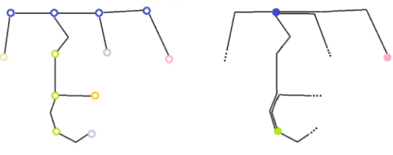
We will need a special case of Theorem 5.1 from [35], illustrated on Figure 1.
Theorem 4.4.([35])Consider an ergodic one-ended unimodular random tree(T, o)of uniformly bounded degrees. Then there is an invariant locally finite tiling inR2 that representsT.
Our original proof of Theorem 4.2 is what we present first. An anonymous referee suggested an alternative proof based on conformal uniformization. We present the main ideas as a 2nd proof. While the second proof also uses parts of the first one, it is more
Figure 1: Representing a tree by a tiling; image taken from [35].
elegant. On the other hand, the first proof seems to be more suitable for quantitative bounds on edge lengths.
Proof of Theorem 4.2, 1st proof. In the following constructions it will often happen that we need to choose some collection of pairwise inner-disjoint curves (broken line seg- ments) connecting some given collection of pairs of points, within some specified bounded domain. We will want to do it so that for a given isometry-invariant and measurable random collection of pairwise disjoint domains in R2 the resulting collection of line segments over all domains is also invariant and measurable. Let us describe a method to do so. For each of the specified bounded domains do the following. Fix a random origin in the domain and two uniformly chosen axes forR2. Then make the choice for the broken line segments so that the pairwise inner-disjointness is satisfied, and every breaking point of every segment has dyadic coordinates of the formh2−k, whereh∈Z andk∈Z+ is minimal such that the choice of all broken line segments with the above constraints is possible. If there is more than one such choice with this minimalk, then choose one of them uniformly at random. So whenever we are making such choices of families of curves, embedded edges etc. in the future, this is how we understand it, without further mention.
Fix some unimodular combinatorial embeddingΣ ={σv : v∈V(G)}ofG(as given by Theorem 2.1), whereσv is the permutation on the edges incident tov∈V(G). Suppose that an embedding of some subgraphH of Gis given, together with an embedding of all the half-edges fromE(G)\E(H). (By an embedding of a half-edge we simply mean the drawing of a broken line segment starting from the vertex, together with a label that tells the other endpoint of the corresponding edge.) We say that this embedding of the edges and half-edges isconsistent withΣ, if the permutation determined by the embedded (half-)edges aroundvin the positive direction isσv.
We will prove a stronger claim than the theorem, namely, that there exists an invariant embedding intoR2that is consistent withΣ.
We may assume thatGhas uniformly bounded degree, as we explain next. We will introduce a new graph G0, that we will obtain fromGby replacing vertices by paths, with two such path adjacent if and only if the original vertices were, and in a way that all degrees inG0 will be at most 3. The construction will give rise to a combinatorial embeddingΣ0 ofG0. Then we will show that an invariant embedding ofG0consistent with Σ0 can be used to define one forGthat is consistent withΣ. The simple construction is summarized on Figure 2. So define G0 as follows. For every vertex v ∈ V(G) let n(v,1), . . . , n(v, k) be the listing of its neighbors given in the order by σv, with the starting neighborn(v,1) chosen at random, wherek = k(v)is the degree ofv. The
vertex setV(G0)will be the union ofv(1), . . . , v(k)over all thev. Now define edges ofG0 as the collection of all pairs{v(i), v(i+ 1)}(asv∈V(G),i= 1, . . . , k(v)−1), and pairs {v(i), w(j)} (asv, w ∈ V(G), n(v, i) = w andn(w, j) = v). By first biasing(G, o)by the degree of the root and then replacing its verticesvby thev(i)(choosing the new root uniformly from the vertices replacing the original one) with edges as inG0, we obtain a rooted graph(G0, o0), which is unimodular (as shown in Example 9.8 of [1] or Subsection 1.4 in [8]). Finally define the unimodular combinatorial embeddingΣ0of(G0, o0): letσv(i)0 be the cyclic permutation v(i−1), w(j), v(i+ 1)
on the neighbors ofv(i)whenever 1< i < k(v), and (trivially) v(2), w(1)
fori= 1and v(k−1), w(k)
fori=k. Suppose we find an invariant embedding consistent withΣ0for the bounded-degree graphG0; let φ(x)be the location of a vertexxby this embedding, and letL(v(i), w(j)) =L(w(j), v(i)) be the drawn edge betweenv(i)andw(j) whenv, w ∈ V(G) and{v(i), w(j)} ∈ E(G0). (Everything that we are doing in the rest of the paragraph is covariant, hence we can fix a representative in the Palm version of the embedded graph and hence refer to actual embedded points.) For everyv∈V(G)pick anιv ∈ {1, . . . , k(v)}at random. The embedded subtree induced byv(1), . . . , v(k)can be used to define broken line segments L(v(i), v(ιv))betweenφ(v(i))andφ(v(ιv)), for alli6=ιv, such that all these broken line segments over the variousv∈V(G)are pairwise inner-disjoint, and also inner-disjoint from all theL(v(i), w(j)),{v(i), w(j)} ∈E(G0),v 6=w. To avoid unnecessary formalism we leave the further details to the interested reader; we only mention that anε-close contour walk around the embedded subtree of edges incident tov(1), . . . , v(k)can give us guidance about where to draw the edges so that the above constraints are satisfied.
DefineL(v(ιv), v(ιv)) =∅. Now, to draw an edge{v, w} ∈ E(G), consider the union of L(v(i), v(ιv)),L(w(j), w(ιw))andL(v(i), w(j)), wheren(v, i) =wandn(w, j) =v. We end up with an embedding ofGfrom the embedding ofG0 as desired; see Figure 2. So from now on we will assume thatGhas bounded degrees.
Figure 2: The scheme of getting an embedding ofGfrom the embedding of its bounded degree versionG0. Dots of the same color stand for thev(1), . . . , v(k(v)), the solid dot indicatesv(ιv).
Now choose a one-ended unimodular spanning treeT ofGand apply Theorem 4.4 to get a tiling representation of it. Ifτ(v)is the tile representingv∈V(T), then we choose a random pointι(v)ofτ(v)to be the embedded image ofv.
For an x ∈ T let Tx be the finite subtree of T induced by the union of all finite components ofT\ {x}and{x}. Say that the depth ofTxiskif the largest distance from xwithinTxisk, and define
Lk :={x∈V(T) :Txhas depthk}.
Ifx, y∈Lk,x6=y, thenTxandTy are disjoint. LetGi be the graph on vertex setV(G) and edge set
E(Gi) :=
{x, y} ∈E(G) : x, y∈Tvfor somev∈Li .
ThenGi is a unimodular finite exhaustion of G. Finally, defineγ(v) = τ(v)whenever v∈L0, and letγ(v)be the ball of radius dist(v, ∂τ(v))/2aroundvwhenv6∈L0. LetΓ(v) be the interior of the closure of∪u∈Tvτ(u).
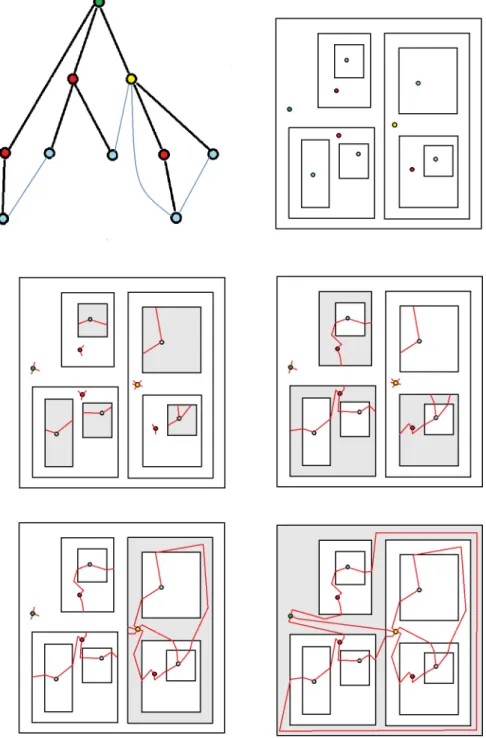
The componentKvof everyv∈LiinGi is such thatG\Kvis connected. Since the vertex set of each such component is that of someTv withv∈Li, the element of highest depth in the component isv, whose depth isi. Furthermore,Γ(v)is simply connected, andι(u)∈Γ(v)for everyu∈V(Kv) =V(Tv). We will embed the edges ofKv inΓ(v), and the above facts guarantee that no two points ofι(V(G\Kv))are separated inR2 by these embedded edges. Furthermore, for all edges not inKvbut incident toKv, we will define an embedded half-edge, connecting the endpoint to∂Γ(v). The procedure is illustrated on Figure 3.
We will proceed in steps, embeddingGn in stepn, and also embedding the half-edges coming fromG\Gn. This will be done in a way that
1. the embedding of Gn is an extension of that of Gn−1. In particular, for every e∈Gn\Gn−1the embedded image ofecontains its embedded half-edges from the previous step, and for every edge ofGn−1the embedding in stepnis the same as in stepn−1.
2. All edges{v, w}withw∈Kv,v∈Ln, are embedded in the interior of the closure ofτ(v)∪Γ(w);
3. similarly, if an edge inE(Kv)\Gn−1has its endpoints in the distinct subtreesTw
andTw0 ofTv, withwandw0 adjacent tov∈Ln, then the edge is embedded into the interior of the closure ofτ(v)∪Γ(w)∪Γ(w0).
4. All half-edges starting from a vertex inKv,v∈Ln, reach∂Γ(v).
As a preparatory step (step 0), consider G0, the empty graph on V(G). For every v∈V(G), pick some embedding of the half-edges starting fromι(v)∈γ(v)to randomly chosen points of the boundary ofγ(v), in a way that the embedding of the half-edges is consistent with Σ. The embedding defined for step 0 trivially satisfies (1)-(4). It is consistent with Σby definition, and any extension will also be consistent with Σ. We proceed to step n recursively. For every component Kv of Gn (v ∈ Ln) do the following. LetKv1, . . . , Kvk be the components ofGn−1induced byV(Kv)(vi∈ ∪n−1j=0Lj).
Then Γ(v) contains the embedded points of V(K), moreover, the Γ(vi) are pairwise disjoint open subsets ofΓ(v)containing the embeddedKvi respectively. Contract every Kvi in Gto a single point, and also contract G\Kv (which is a connected graph) to a single pointx∞. The resulting finite graph K0 inherits a combinatorial embedding fromΣ. Consider an arbitrary embedding ofK0 to the 2-sphere that represents this combinatorial embedding. Remove an infinitesimally small neigborhood of the embedded nodes, to get a 2-sphere with holes in it and pairwise disjoint arcs connecting some of these holes. It is easy to check that there is a homeomorhism from this surface toτ(v), which maps the boundary of the hole belonging to x∞ to∂Γ(v)⊂∂τ(v), and maps the boundary of the hole corresponding to the contractedKvito∂Γ(vi)⊂∂τ(v). Furthermore, this homeomorphism can be chosen so that the images of the drawn segments are continuations of the respective drawn half-edges in theΓ(vi). We have just shown that there exists an embedding of the componentKvofGn intoΓ(v)that satisfies (1)-(4); now choose the broken line segments for one such embedding randomly in a way as described at the beginning of this proof.
Figure 3: A subtreeTv ofT is taken (as the tree of Figure 1, with vertices recolored), together with the other edges ofGinduced by it, producing the componentKv ofGn. Blue vertices are inL0, red ones inL1, yellow is forL2, green forL3. The embedding of edges is shown over several steps. Shaded areas indicate theτ(w),w∈Li, where edges are drawn in stepi. They are not used in any later step.
Since every step is an extension of the previous one, we obtain an embedding ofGin the limit, as desired. Local finiteness is guaranteed by the fact that everyτ(u)(u∈V(G)) is intersected by finitely many embedded edges.
Proof of Theorem 4.2, sketch of 2nd proof. Up until Figure 2, we proceed as in the 1st proof, that is, we choose a one-ended spanning treeT ofGand choose some unimodular combinatorial embedding ofG. Also consider an invariant spanning biinfinite pathP of Z2, e.g. the UST Peano path. The complement of the path inR2consists of two simply connected domains. Pick one of them at random and consider a conformal map from this domain to the upper half plane such that its extension to the closure maps the origin to the origin. This map is unique up to scaling; fix one of them and call itφ. The points of P are mapped to points of the real line, and their images inherit the ordering coming from the path. Using the fixed combinatorial embedding ofG(and hence ofT), there is a well-defined contour walk aroundT; starting this walk to the left and to the right from the root we can define a surjective map fromφ(V(P))toV(T), with 0 mapped to the root. Ifv∈V(T)is a leaf, that is, if it only has one preimage by this map, call this preimageψ(v); otherwisevhas a leftmost and rightmost preimage, and we take the top of the circular half-circle on these two points to beψ(v). We can draw all the edges ofT between the respectiveψ(v)as geodesic segments in the (Poincaré) halfplane, and no crossing will happen by construction. Thenφ−1defines an embedding ofT intoR2that is unimodular, and applying a random isometry ofR2that maps 0 to some point of the unit square makes everything isometry-invariant.
The embedding ofT is consistent with the given combinatorial embedding, hence it can be extended to an embedding ofG(which is not necessarily invariant yet). Now, the complement of the embedded tree is itself conformally a halfplane. One can draw in the additional edges ofGas the conformal geodesics between the relevant points on the boundary of the tree, to end up with an invariant embedding ofG. To have broken line segments represent the embedded edges, one can replace the curves by suitable approximations.
Theorem 4.5.Every amenable unimodular random planar graph(G, o)can be repre- sented inR2as the neighborhood graph of an invariant random tiling.
In [35] it is proved that every amenable unimodular transitive graph can be repre- sented by an invariant tiling ofRd ford≥3, and the proof extends from transitive to random right away.
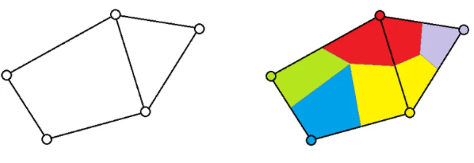
Proof. Consider the embedding ofGintoR2as in Theorem 4.2 and letP be the point process that the embedded vertices define. To each faceFand pointv∈∂F,v∈ P, we will assign a piece of the face incident tov, in such a way that two such pieces share a 1-dimensional boundary iff the corresponding vertices are adjacent. For the case of bounded faces one can apply a modified “barycentric subdivision”, see Figure 4: for each pairvandwof adjacent vertices that are consecutive alongF, consider the broken line segment representing the edge between them, and consider its midpoint, that is, the point that halves the length of the broken line. Choose some point uniformly inF, and connect it to all these midpoints by some broken line. IfF is infinite, we will apply a trick similar to the one in [24]. For every pairvandwof adjacent vertices such thatι(v) andι(w)are consecutive alongF, leth(v, w) =h(w, v)be the midpoint of the broken line segment between them. Choose a conformal mapf betweenF and the upper half plane HofCthat maps infinity to infinity. By the standard extension off−1to the boundary
∂H, we can define a set off-images inRfor everyh(v, w)∈∂F. (This set consists of one or two points, depending on whether the broken line betweenv andwhasF on only one side or on both.) Leta∈Rbe one such image, and consider the vertical line La ={a+bi : b∈R+}inH. Considerf−1(La)for all thea. One can check that they subdivideF into pieces as we wanted. It is also clear that the construction does not depend on the choice off (which is unique up to conformal automorphisms of the upper
half plane of the formx7→ax+b,a, b∈R,a6= 0), and that it is invariant. See [24] for a detailed argument.
Figure 4: Splitting up a face to subtiles. Broken line segments are represented by straight segments for simplicity.
It remains to prove that the tile of the origin has finite area almost surely. This is known for any invariant point process inR2(whose intensity is automatically positive) and partition as in our setup, see, e.g., (9.15) in [10].
We expect that with some extra work one could also get a tiling where every tile has area 1. One would have to ensure that the embedded vertices in Theorem 4.2 form a point process where the number of points in large boxes is relatively close to the expectation, and then build up the tiling stepwise and directly, eventually assigning unit tiles to all vertices. We have not worked out the details.
What seems to be harder to control, is the diameter of the tiles.
Question 4.6.What can we say about the distribution of the diameter of a tile in a construction as Theorem 4.5? How fast can it decay?
Various invariance principles follow from [14] if one is able to construct an initial embedding for the given graph that satisfies a certain finite energy condition. The embeddings are assumed to be translation invariant modulo scaling. Whether our method can be useful in this setting is to be investigated in the future.
5 Proofs of the main theorems
Proof of Theorem 1.1. The existence of such representations ifGis amenable is proved in Theorems 4.2 and 4.5.
For the “only if” part, suppose first that a nonamenableGhad an isometry-invariant embedding as in Theorem 1.2 intoR2. Then one could use the invariant random partitions ofR2to2ntimes2nsquares to define a unimodular finite exhaustion ofG. ThusGhas to be amenable, a contradiction.
Proof of Theorem 1.2. For the nonamenable case the unimodular embedding intoH2is given in Theorem 3.1. That there is no such an embedding intoR2is proved the same way as in the proof of Theorem 1.1.
If Gis amenable, an isometry-invariant embedding intoR2 exists. With the same arguments as in Example 9.5 of Aldous and Lyons in [1], the Palm version of this random embedded graph (as a graph with the decoration given by the embedding and rooted in the origin) is unimodular.
Proof of Theorem 1.3. The “if” parts of the claims follow from Theorem 4.5 and 3.1.
(Although Theorem 3.1 is for simple graphs, the tiling obtained from a circle-packing can be extended when there are parallel edges or loops.)
For the “only if” part, note that an invariant tiling gives rise to an invariant embedding (choose a uniform random point in each tile and suitably connect it to its neighbors).
Hence the claim is reduced to that in Theorem 1.2.
References
[1] D. Aldous and R. Lyons, Processes on unimodular random networks. Electron. J. Probab. 12 (2007) 1454–1508. MR-2354165
[2] O. Angel, T. Hutchcroft, A. Nachmias and G. Ray, Unimodular hyperbolic triangulations: circle packing and random walk. Invent. Math. 206 (2016) 229–268. MR-3556528
[3] O. Angel, T. Hutchcroft, A. Nachmias and G. Ray, Hyperbolic and parabolic unimodular random graphs. Geom. Funct. Anal. 28 (2018) 879–942. MR-3820434
[4] O. Angel and O.Schramm, Uniform infinite planar triangulations. Comm. Math. Phys. 241 (2003) 191–213. MR-2013797
[5] F. Baccelli, MO. Haji-Mirsadeghi, A. Khezeli, Unimodular Hausdorff and Minkowski dimen- sions. Preprint (2018).arXiv:1807.02980
[6] I. Benjamini and N. Curien, Ergodic theory on stationary random graphs. Electron. J. Probab.
17 (2012) 1–20. MR-2994841
[7] I. Benjamini and O. Schramm, Percolation in the hyperbolic plane. J. Amer. Math. Soc. 14 (2001) 487–507. MR-1815220
[8] D. Beringer, G. Pete and Á. Timár, On percolation critical probabilities and unimodular random graphs. Electron. J. Probab. 22 (2017) 1–28. MR-3742403
[9] M. Bonk and O. Schramm, Embeddings of Gromov hyperbolic spaces. Geom. Funct. Anal. 10 (2000) 266–306. MR-1771428
[10] S.N. Chiu, D. Stoyan, W.S. Kendall, and J. Mecke,Stochastic geometry and its applications, 3rd edition. John Wiley & Sons (2013). MR-3236788
[11] A. Connes, J. Feldman and B. Weiss, An amenable equivalence relation is generated by a single transformation. Ergodic Theory and Dynamical Systems, 1(4) (1981) 431–450. MR-0662736 [12] P.A. Ferrari, C. Landim and H. Thorisson, Poisson trees, succession lines and coalescing random walks. Ann. Inst. H. Poincaré Probab. Statist. 40(2) (2004) 141–152. MR-2044812 [13] O. Gurel-Gurevich, D.C. Jerison and A. Nachmias, The Dirichlet problem for orthodiagonal
maps. Adv. Math. 374 (2020) 107379. MR-4157579
[14] E. Gwynne, J. Miller and S. Sheffield, An invariance principle for ergodic scale-free random environments. Preprint (2018).arXiv:1807.07515v2
[15] J. Haslegrave and C. Panagiotis, Site percolation and isoperimetric inequalities for plane graphs. Random Struct. Algorithms 58, no. 1 (2021) 150–163. MR-4180256
[16] Z-X. He and O. Schramm, Fixed points, Koebe uniformization and circle packings. Annals of Math. 137 (1993) 369–406. MR-1207210
[17] Z-X. He and O. Schramm, Hyperbolic and parabolic packings. Discrete Comput. Geom. 14 (1995) 123–149. MR-1331923
[18] M. Heveling and G. Last, Characterization of Palm measures via bijective point-shifts. Ann.
Probab. 33 (5) (2005) 1698–1715. MR-2165576
[19] A. Holroyd, Geometric properties of Poisson matchings. Probab. Theory Related Fields, 150 (2011) 511–527. MR-2824865
[20] A.E. Holroyd and Y. Peres, Trees and matchings from point processes. Elect. Comm. in Probab.
8 (2003) 17–27. MR-1961286
[21] A.E. Holroyd and Y. Peres, Extra heads and invariant allocations. Ann. Probab. Volume 33, Number 1 (2005) 31–52. MR-2118858
[22] A.E. Holroyd, R. Pemantle, Y. Peres and O. Schramm, Poisson matching. Ann. Inst. H. Poincaré Probab. Statist. 45(1) (2009) 266–287. MR-2500239
[23] A. Khezeli, Counter examples to invariant circle packing. Preprint (2019).
arXiv:1912.12862v1
[24] M. Krikun, Connected allocation to Poisson points inR2. Electron. Commun. Probab. 12 (2007) 140–145. MR-2318161
[25] G. Last and M. Penrose,Lectures on the Poisson Process, Cambridge University Press (2017).
MR-3791470
[26] L. Lovász,Large networks and graph limits, volume 60 ofColloquium Publications, Amer.
Math. Soc., Providence, RI (2012). MR-3012035
[27] R. Lyons and Y. Peres,Probability on Trees and Networks, Cambridge University Press, New York (2016). Available at http://pages.iu.edu/~rdlyons/, MR-3616205
[28] J. Mecke, Invarianzeigenschaften allgemeiner Palmscher Masse. Math. Nachr. 65 (1975) 335–344. MR-0374385
[29] A. Nachmias,Planar Maps, Random Walks and Circle Packing, École d’Été de Probabilités de Saint-Flour XLVIII – 2018, (2018). MR-3970273
[30] V.G. Pestov, Hyperlinear and sofic groups: a brief guide. Bull. Symbolic Logic 14(4) (2008) 449–480. MR-2460675
[31] O. Schramm, Rigidity of infinite (circle) packings. J. Amer. Math. Soc. 4 (1991) 127–149.
MR-1076089
[32] H. Thorisson,Coupling, Stationarity, and Regeneration, Springer (2000). MR-1741181 [33] W.P. Thurston,Three-dimensional geometry and topology, Princeton university press (1997).
MR-1435975
[34] Á. Timár, Tree and Grid Factors of General Point Processes. Electron. Commun. Probab. 9 (2004) 53–59. MR-2081459
[35] Á. Timár, A nonamenable “factor” of a Euclidean space. Ann. Probab., to appear (2021).
arXiv:1712.08210v1, MR-4255149
[36] Á. Timár, Unimodular random planar graphs are sofic. Preprint (2019).arXiv:1910.01307v1 [37] Á. Timár, One-ended spanning trees in amenable unimodular graphs. Electron. Commun.
Probab. 24 (2019) 1–12. MR-4040939
[38] Á. Timár and L. Tóth, A full characterization of invariant embeddability of unimodular planar graphs. Preprint (2021).arXiv:2101.12709, MR-4141357
Acknowledgments. We are indebted to an anonymous referee for many valuable improvements on the paper, as well as for finding an error and suggesting some ideas for the correction. We thank another referee for the suggestion of the 2nd proof for Theorem 4.2. Thanks to Gábor Pete, Omer Angel, Sebastien Martineau, Romain Tessera and Ron Peled for useful discussions, and to András Stipsicz for a reference.
![Figure 1: Representing a tree by a tiling; image taken from [35].](https://thumb-eu.123doks.com/thumbv2/9dokorg/734979.29585/11.892.257.628.168.333/figure-representing-tree-by-tiling-image-taken-from.webp)