AN ANALOGUE OF A THEOREM OF STEINITZ FOR BALL POLYHEDRA IN R3
SAMI MEZAL ALMOHAMMAD , ZSOLT L ´ANGI, AND M ´ARTON NASZ ´ODI
Abstract. Steinitz’s theorem states that a graphGis the edge-graph of a 3-dimensional convex polyhedron if and only if,Gis simple, plane and 3-connected. We prove an ana- logue of this theorem for ball polyhedra, that is, for intersections of finitely many unit balls inR3.
1. Introduction
Our work takes place in Euclidean 3-space. For the closed ball of radius ρ centered at x ∈ R3, we use the notation B[x, ρ] := {y ∈ R3 : d(x, y) ≤ ρ}. The 2-dimensional sphere (the boundary of a closed ball) is denoted by S2(x, ρ) :={y∈ R3 : d(x, y) =ρ}. For brevity, we set B[x] := B[x,1], S(x) := S2(x,1) and for a set X ⊆ R3, we write B[X] := T
x∈X
B[x].
Let X ⊂ R3 be a finite, nonempty set contained in a ball of radius less than 1. The set P = B[X] is called a ball polyhedron. For any x ∈ X, we call B[x] a generating ball of P and S(x) a generating sphere of P. Unless we state otherwise, we will assume that X is a reduced set of centers, that is, that B[X]6=B[X\ {x}] for any x∈X.
The face structure of a 3-dimensional ball polyhedron B[X] are defined in a natural way: a point on the boundary of B[X] belonging to at least three generating spheres is called avertex; a connected component of the intersection of two generating spheres and B[X] is called an edge, if it is a non-degenerate circular arc; and the intersection of a generating sphere and B[X] is called a face.
The face structure of a ball polyhedron, unlike that of a convex polyhedron, is not neces- sarily an algebraic lattice, with respect to containment, see [BN06]. Following [BLNP07], we call a ball polyhedron inR3 standard, if its vertex-edge-face structure is a lattice with respect to containment. This is the case if, and only if, the intersection of any two faces is either empty, or one vertex or one edge, and any two edges share at most one vertex. The paper [KMP10] and Chapter 6 of the beautiful book [MMO19] by Martini, Montejano and Oliveros provide further background on the theory of ball polyhedra.
A fundamental result of Steinitz (see, [Zie95], [SR34] and [Ste22]) states that a graph Gis the edge-graph of a 3-dimensional convex polyhedron if and only if, Gis simple (ie., it contains no loops and no parallel edges), plane and 3-connected (ie., removing any two vertices and the edges adjacent to them yields a connected graph). In [BLNP07], it is shown that the edge-graph of any standard ball polyhedron in R3 is simple, plane and 3-connected. Solving an open problem posed in [BLNP07] and [Bez13], our main result shows that the converse holds as well.
Theorem 1. Every 3-connected, simple plane graph is the edge-graph of a standard ball polyhedron in R3.
2010Mathematics Subject Classification. 52B10, 52A30, 52B05.
Key words and phrases. Steinitz’s theorem, polyhedron, ball polyhedron, edge-graph.
1
arXiv:2011.10105v1 [math.MG] 19 Nov 2020
The proof of Steinitz’s theorem consists of two parts. First, it is shown that 3- connected, simple plane graphs can be “reduced” by a finite sequence of certain graph operations to the complete graph K4 on four vertices. Second, in the geometric part, it is shown that if a graph Gis obtained from another graph G0 by such an operation and G is realizable as the edge-graph of a polyhedron, then G0 is realizable as well. To prove Theorem 1, we use the first, combinatorial part without modification. Our contribution is the proof of the second, geometric part in the setting of ball polyhedra.
The structure of the paper is the following. First, in Section 2, we introduce these op- erations on graphs, and recall facts on the face structure of the dual of a ball polyhedron.
In Section 3, we state our main contribution, Theorem 2, which shows the “backward inheritance” of realizability by ball polyhedra under these graph operations, and deduce Theorem 1 from it. Finally, in Section 4, we prove Theorem 2.
2. Preliminaries
2.1. Simple ∆-to-Y and Y-to-∆ reductions on a plane graph. Let G be a 3- connected plane graph andK3 be a triangular face with verticesv1, v2 and v3 (resp.,K1,3
be a subgraph consisting of a 3-valent vertexv ofG, its neighborsv1, v2, v3, and the edges {v, vi}connecting v to its neighbors). A ∆Y operation is defined as the graph operation which removes the edges {vi, vj} of a triangular face K3, adds a new vertex v from the face, and connects it tovis, or vice versa, it takes a subgraphK1,3 ofG, removes the vertex v and the edges incident to it, then connects all pairs v −I, vj by an edge. To specify the direction of the transformation, we will distinguish between a ∆-to-Y transformation and a Y-to-∆ transformation (see Figure 1).
v1
v2 v3
K3
v1
v2 v3
⇐⇒
vK1,3
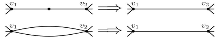
Figure 1. =⇒: A ∆-to-Y transformation;⇐=: A Y-to-∆ transformation A ∆Y operation may create multiple edges or vertices of degree two. A graph with such objects is clearly not the edge-graph of a standard ball polyhedron. To fix these issues, we define the following notion. A series-parallel reduction, or SP-reduction is the replacement of a pair of edges incident to a vertex of degree 2 with a single edge or, the replacement of a pair of parallel edges with a single edge that connects their common endpoints, see Figure 2.
v1 v2
= ⇒
v1 v2v1 v2
= ⇒
v1 v2Figure 2. Examples of SP-reductions
Assume that a graph Gcontains K1,3 as a subgraph whose degree 3 vertex is denoted by v, and its neighbors are v1, v2, v3 (resp., K3 with verticesv1, v2, v3), see Figure 1. We
2
call edges of G that connect two vertices of K1,3 (resp., K3) internal edges. We define the outer degree of a neighbor ofv (resp., a vertex of K3), as the number of non-internal edges adjacent to it. A K1,3 is called Y0, Y1, Y2, or Y3 if it has zero, one, two, or three internal edges respectively. A K3 is called ∆0, ∆1, ∆2, or ∆3 if it has zero, one, two, or three vertices of outer degree one, respectively.
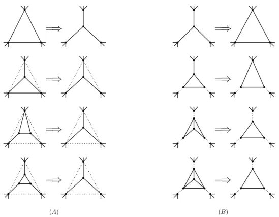
Asimple ∆Y reduction means any ∆Y operation followed immediately by SP-reductions that are then possible. There are four different types of simple ∆-to-Y and Y-to-∆ re- ductions (cf. Corollary 4.7 of [Zie95]), as shown in Figure 3.
Proposition 2.1. Every 3-connected plane graph G can be reduced to K4 by a sequence of simple ∆Y reductions.
= ⇒ = ⇒
= ⇒ = ⇒
= ⇒ = ⇒
= ⇒
(A)
= ⇒
(B)
Figure 3. (A) Four types of simple ∆-to-Y reduction, and (B) four types of simpleY-to-∆ reduction, where the dotted lines denote edges that may or may not be present, and are not affected by the simple ∆-to-Y and Y-to-∆ reductions.
2.2. Standard graphs. A planar graph with a fixed drawing on the plane is called a plane graph. It is well known that 3-connected planar graphs have only one drawing, that is, all plane drawings of such a graph have isomorphic face lattices [Zie95, Section 4.1].
Definition 2.1. Let G be a plane graph. We call G standard, if
(i) the intersection of any two faces is either empty, or one vertex or one edge, and (ii) any two edges share at most one vertex.
Remark 2.1. Let G be the edge-graph of a ball polyhedron. Then G is standard if and only if the ball polyhedron is a standard ball polyhedron.
We leave the proof of the following two lemmas to the reader as an exercise.
3
Lemma 2.1. Let G be a 3-connected plane graph and let the graph G0 be derived from G by a simple ∆-to-Y reduction. If G is a standard graph, then so is G0.
The subdivision of an edge {t1, t2} of a graph Gis another graph obtained from Gby removing the edge {t1, t2}, then adding a new vertex t0 and, finally, adding the edges {t1, t0} and {t0, t2}.
Lemma 2.2. Let G be a standard graph, E be a face of G and {u1, u3}, {u3, u2} be two edges of E such that u1 and u2 are non-adjacent vertices.
I. If the graphH is obtained fromGby adding the edge{u1, u2}, thenH is a standard graph.
II. If the graph H0 is obtained from G by adding the edge {u2, u0} where u0 is a new vertex subdividing the edge {u1, u3}, then H0 is a standard graph.
III. If the graph H00 is obtained from G by adding the edge {u0, u00} where u0 and u00 are two new vertices subdividing the edges {u1, u3} and{u3, u2} respectively, then H00 is a standard graph.
2.3. Graph duality. We denote the dual of a plane graph G by G?, see [Zie95, Sec- tion 4.1]. It is well known that G? is also a plane graph, and G? is 3-connected if and only if, Gis 3-connected.
According to the following fact, simple ∆-to-Y reductions and simple Y-to-∆ reduc- tions are dual to each other, see [Zie95, Section 4.2].
Proposition 2.2. LetGandG0 be 3-connected plane graphs. ThenG0 is obtained fromG by a simple ∆-to-Y reduction if and only if, G0? is obtained from G? by a simple Y-to-∆
reduction.
2.4. The dual of a ball polyhedron. In the following, F(B[X]) denotes the set of faces, and V(B[X]) denotes the set of vertices of the ball polyhedron B[X].
LetB[X] be a ball polyhedron inR3 all of whose faces contain at least three vertices.
In [BN06], the dual of B[X] is introduced as the ball polyhedron B[V(B[X])], and a bijection, called the duality mapping between B[X] and B[V(B[X])], is given between the faces, edges and vertices of B[X] and B[V(B[X])], consisting of the following three mappings:
(1) The vertex-face mapping is
V(B[X])3v 7→V ∈ F(B[V(B[X])])
whereV is the face of B[V(B[X])] withv as its center.
(2) The face-vertex mapping is
F(B[X])3F 7→f ∈ V(B[V(B[X])])
wheref is the center of the sphere supporting the face F.
(3) Theedge-edgemapping is the following. Two vertices inB[V(B[X])] are connected by an edge if and only if, the corresponding faces of B[X] meet in an edge.
Note that every face of a standard ball polyhedron contains at least three edges. The relationship between graph duality and duality of ball polyhedra is described below.
Lemma 2.3 (Theorem 6.6.5., [Bez13]). LetP be a standard ball polyhedron of R3. Then the intersectionP? of the closed unit balls centered at the vertices of P is another standard ball polyhedron whose face lattice is dual to that of P.
3. Proof of Theorem 1 Our main contribution follows.
4
Theorem 2. Let G0 be a 3-connected plane graph, and let the graph G be derived from G0 by a simple Y-to-∆ reduction. If G is the edge-graph of a standard ball polyhedron in R3, then so is G0.
First, we show how Theorem 2 implies Theorem 1.
Proof of Theorem 1. LetGbe a 3-connected simple plane graph. By Proposition 2.1, the graph Greduces toK4 the edge-graph of the standard ball tetrahedron by a sequence of simple ∆Y reductions.
Now we show that the standard ball tetrahedron can be gradually turned into a real- ization of G. Let H be the edge-graph of a standard ball polyhedron and assume that H is obtained from another edge-graphH0 by a simple ∆Y reduction. We want to show that H0 is realized by a standard ball polyhedron. So we need to discuss two cases:
First, assume that H is obtained from H0 by a simple Y-to-∆ reduction. Then by Theorem 2, H0 is realized by a standard ball polyhedron.
Second, assume that H is obtained from H0 by a simple ∆-to-Y reduction. Then by Proposition 2.2, we get that the edge-graph H? is obtained from the edge-graph H0? by a simpleY-to-∆ reduction. By Lemma 2.3, the edge-graph H? is realized by a standard ball polyhedron, and by Theorem 2, the edge-graph H0? is realized by a standard ball polyhedron. Again by Lemma 2.3, the edge-graph H0 is realized by a standard ball
polyhedron, and this completes the proof.
dual
H0 simple ∆-to-Y H
By assumption,H is the edge-graph of a standard ball-polyhedron.
H0?simpleY-to-∆ H?
dual dual
By Lemma 2.3, H? is the edge-graph of a standard ball-polyhedron.
By Theorem 2,H0? is the edge-graph of a standard ball-polyhedron.
By Lemma 2.3,H0is the edge-graph of a standard ball-polyhedron.
4. Proof of Theorem 2
Let ∅ 6= X ⊂ R3 be a finite set and B[X] be a standard ball polyhedron with edge- graph G, and assume that Gis obtained from a graph G0 by a simpleY-to-∆ reduction.
We need to show that G0 is realized by a standard ball polyhedron.
Let Λ denote the triangular face of B[X] which realizes the triangle obtained in the Y-to-∆ reduction, let S(xΛ) be its supporting unit sphere, and v1, v2, v3 be the vertices of Λ and e1,e2,e3 the edges. LetF1,F2 and F3 denote the faces ofB[X] distinct from Λ containing e1, e2 and e3 respectively, and let S(x1), S(x2) and S(x3) be the unit spheres supporting these faces, see Figure 4.
The starting point of the proof of Theorem 2 is the removal of the ball that generates the triangular face Λ. Thus, we obtain another ball polyhedron, B[X \ {xΛ}]. The following lemma (which we prove later) describes the edge-graph of B[X \ {xΛ}] and, combined with Lemma 2.1 yields that it is a standard graph, and hence, by Remark 2.1, B[X\ {xΛ}] is a standard ball polyhedron.
Lemma 4.1. The edge-graph of the ball polyhedron B[X\ {xΛ}] is obtained by a simple
∆-to-Y reduction applied to Λ in the role of K3.
5
F1 e1 e2 F2
F3
e3
Λ v3
v2 v1
Figure 4.
The edge-graph of B[X\ {xΛ}] described in Lemma 4.1 may be G0, in which case we are done. However, it may happen that this is not G0, more precisely, the graph G is derived from G0 by a simple Y-to-∆ reduction, but the converse is not always true, it may happen that G0 is not derived from G by a simple ∆-to-Y reduction. The reason is that when we do a ∆-to-Y reduction, the vertices of the triangle of outer degree one inG become degree two vertices in the graph obtained from G by a ∆-to-Y reduction. Next, we do the SP-reduction, and these vertices are lost, see Figure 5 (C) and (D). Moreover, the internal edges will be missing as well, see Figure 5 (B), (C) and (D).
The following lemma describes how the edge-graph of B[X \ {xΛ}] is converted into G0 by adding the missing vertices and edges. We achieve this by adding some extra balls. Lemma 2.2 yields thatG0 is a standard graph, and hence, by Remark 2.1, the ball polyhedron realizing G0 is a standard ball polyhedron.
(A)
= ⇒
Y-to-∆
c
v2 v3
v1
= ⇒
∆-to-Y
v2 v3
v1
c
v2 v3
v1
(B)
= ⇒
Y-to-∆
c
v2 v3
v1
= ⇒
∆-to-Y
v2 v3
v1
c
v2 v3
v1
(C)
= ⇒
Y-to-∆
v2 v3
c v03 v1
= ⇒
∆-to-Y
v2 v3
v03 v1
v2
c v30 v1
(D)
= ⇒
Y-to-∆
v2 v3
c
v02 v03
v1
= ⇒
∆-to-Y
v2 v3
v02 v30
v1
c
v20 v30
v1
Figure 5.
6
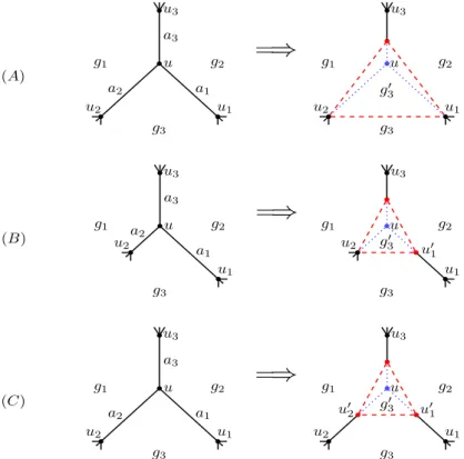
Lemma 4.2. Let ∅ 6=Z ⊂R3 be a finite set and B[Z] be a ball polyhedron. If the edge- graph of B[Z] contains Y0 as an induced subgraph whose vertices are u, u1, u2 and u3, and whose edges are a1, a2 and a3, see Figure 6, left side, then
I. there exists a center w such that the edge-graph of the ball polyhedronB[Z∪ {w}] is obtained from the edge-graph ofB[Z] by adding the internal edge {u1, u2}. II. there exists a center w0 such that the edge-graph of the ball polyhedronB[Z∪{w0}]
is obtained from the edge-graph of B[Z] by adding the edge {u2, u01}, where u01 is a new vertex subdividing the edge a1.
III. there exists a centerw00 such that the edge-graph of the ball polyhedronB[Z∪{w00}] is obtained from the edge-graph of B[Z] by adding the edge{u01, u02}, where u01 and u02 are two new vertices subdividing the edges a1 and a2 respectively.
In summary, proving Lemmas 4.1 and 4.2, we prove Theorem 2, which in turn yields Theorem 1.
4.1. Proof of Lemma 4.1. In this section, we use the notation of Lemma 4.1 and Figure 4.
The following claim is obvious.
Claim 4.1. For any i∈ {1,2,3}, Λ\ei is contained in the interior of B[xi].
The following claim is the key of our proof. It states that the “new part” of the boundary of the new ball polyhedron B[X \ {xΛ}] belongs to the union of S(x1), S(x2) and S(x3).
Claim 4.2. bd(B[X0])\bd(B[X])⊆S(x1)∪S(x2)∪S(x3), where X0 =X\ {xΛ}. Proof. Consider a pointq∈bd(B[X0])\bd(B[X]). Then there exists a generating sphere S(xq) ofB[X0] such thatq ∈S(xq) andxq ∈X0, implying thatS(xq) is a generating sphere of B[X] as well. Let F =S(xq)∩B[X] and F0 = S(xq)∩B[X0]. ThenF =F0∩B[xΛ], F ⊆F0,q∈F0, andq /∈F. This yields thatF0∩S(xΛ) is a non-degenerate circular arc in F0 that separatesq fromF. Thus F intersects Λ in a non-degenerate circular arc. That only happens ifF intersects Λ in an edge of B[X], and hence,xq =x1, x2, or x3.
The following Claim is obvious.
Claim 4.3. Let B1,B2 and B3 be closed unit balls in R3 such that B1 ∩B2 ∩B3 is a ball polyhedron with three faces. Then B1∩B2∩B3 is a ball polyedron with two vertices connected by three edges.
Finally, we are in the position to prove Lemma 4.1. By Claim 4.3, the boundary of B[x1]∩B[x2]∩B[x3] contains two vertices of degree three say q and ¯q, three edges, and three faces. We need to prove that the “new part” N := bd(B[X\ {xΛ}])\bd(B[X]) of the boundary of the ball polyhedron B[X\ {xΛ}] contains either q or ¯q with part from each of the three edges, and part from each of the three faces (i.e., K1,3). It means that when we remove the ballB[xΛ], the triangular face Λ ofG will be replaced by Y0 =K1,3 in the edge-graph of B[X\ {xΛ}], i.e., the edge-graph of B[X\ {xΛ}] is derived from G by a simple ∆-to-Y reduction.
Let Γ :=B[x1]∩B[x2]∩B[x3] andγ := bd(Λ) =e1∪e2∪e3, see Figure 4. By Claim 4.2, N ⊆S(x1)∪S(x2)∪S(x3), this implies thatN ⊆ bd(Γ). Clearly, bd(Γ) has three edges, say e01, e02 and e03 such that e01 ⊆S(x2)∩S(x3), e02 ⊆S(x1)∩S(x3) ande03 ⊆S(x1)∩S(x2).
By Claim 4.1,vi ∈int (B[xi]) for all i= 1,2,3. By Claim 4.3, S(x1)∩S(x2)∩S(x3) is a set of two points q and ¯q. Clearly, {v1, v2, v3} ∩ {q, q¯}=∅.
7
Since e01\ {q, q¯} ⊆ int(B[x1]), v1 ∈ e01\ {q, q¯} and {e02, e03} ⊆ S(x1), this implies that v1 belongs to e01 \ {q, q¯} and does not belong to e02 or to e03. Similarly, vi belongs to e0i\ {q, q¯}(i= 2,3) only, respectively. Thus, exactly one of v1, v2 and v3 is contained on each of the three edges of Γ.
Observe that both S(xΛ)∩Γ and Λ are the intersections of three spherical disks on S(xΛ), each smaller than a hemi-sphere: S(xΛ)∩B[x1],S(xΛ)∩B[x2] andS(xΛ)∩B[x3].
Hence, S(xΛ)∩Γ = Λ, and it follows that S(xΛ)∩bd(Γ) =γ.
It follows that γ partitions bd(Γ) into two components, q is in one component and ¯q is in the other, we may assume that ¯q ∈ int (B[xΛ]). Claim 4.2 yields that q ∈ N as required. This completes the proof of Lemma 4.1.
4.2. Proof of Lemma 4.2.
(I) Let g1, g2 and g3 be the faces of B[Z] such that a1 = g2 ∩g3, a2 = g1 ∩g3 and a3 = g1 ∩g2 and let S(z1), S(z2) and S(z3) be the spheres supporting these faces, see Figure 6, left side.
To add an internal edge toY0, we will add a rotated copyz30 ofz3 to the setZ, where the axis of the rotation is the line through u1 and u2, the angle of the rotation is sufficiently small, and u is outside of B[z30]. Thus, we obtain a new triangular face g30 supported by S(z30), see the dashed lines on Figure 6 (A), and remove the dotted lines on Figure 6 (A).
(A)
= ⇒
g3
g2
g1
a3
a1
a2
u
u2 u1
u3
g3
g03
g2
g1 u
u2 u1
u3
(B)
= ⇒
g3
g2
g1
a3
a1
a2 u u2
u1
u3
u01 g03
g3
g2
g1 u
u2
u1
u3
(C)
= ⇒
g3
g2
g1
a3
a1
a2
u
u2 u1
u3
g03
g3
g2
g1
u02 u01 u
u2 u1
u3
Figure 6. The dotted (blue) vertices and edges are removed and the dashed (red) vertices and edges are introduced in the new graph.
(II) To add a new vertex and a new edge to Y0, we use the same method as in (I), but we choose the rotation axis so that it passes through the vertexu2 and intersects the edge a1 at a point, say u01, distinct from its endpoints, see Figure 6 (B).
(III) To add two new vertices and a new edge to Y0, we use again the same method of (I), but this time, we choose the rotation axis so that it intersects the edges a1 anda2 at
8
two points, say u01 and u02 respectively, distinct from their endpoints, see Figure 6 (C).
This finishes the proof of Lemma 4.2.
Acknowledgements
SMA would like to thank the Tempus Public Foundation (TPF), Stipendium Hungar- icum program, and University of Thi-Qar, Iraq for the support for his PhD scholarship.
ZL was supported by grants K119670 and BME Water Sciences & Disaster Prevention TKP2020 IE of the National Research, Development and Innovation Fund (NRDI), by the ´UNKP-20-5 New National Excellence Program of the Ministry for Innovation and Technology, and the J´anos Bolyai Scholarship of the Hungarian Academy of Sciences.
MN was supported by the National Research, Development and Innovation Fund (NRDI) grant K119670, by the ´UNKP-20-5 New National Excellence Program of the Ministry for Innovation and Technology from the source of the NRDI, as well as the J´anos Bolyai Scholarship of the Hungarian Academy of Sciences.
References
[Bez13] K´aroly Bezdek,Lectures on sphere arrangements-the discrete geometric side, Springer, 2013.
[BLNP07] K´aroly Bezdek, Zsolt L´angi, M´arton Nasz´odi, and Peter Papez,Ball-polyhedra, Discrete Com- put. Geom.38(2007), no. 2, 201–230. MR 2343304
[BN06] K´aroly Bezdek and M´arton Nasz´odi,Rigidity of ball-polyhedra in Euclidean 3-space, European Journal of Combinatorics27(2006), no. 2, 255 – 268.
[KMP10] Y. S. Kupitz, H. Martini, and M. A. Perles, Ball polytopes and the V´azsonyi problem, Acta Math. Hungar.126(2010), no. 1-2, 99–163. MR 2593321 (2011b:52025)
[MMO19] Horst Martini, Luis Montejano, and D´eborah Oliveros, Bodies of constant width, Birkh¨auser/Springer, Cham, 2019, An introduction to convex geometry with applications.
MR 3930585
[SR34] Ernst Steinitz and Hans Rademacher, Vorlesungen ¨uber die theorie der polyeder, Springer- Verlag, 1934.
[Ste22] Ernst Steinitz, Polyeder und raumeinteilungen, encyclop¨adie der mathematischen wis- senschaften, vol. 3, 1922.
[Zie95] G.M. Ziegler,Lectures on polytopes, Graduate texts in mathematics, Springer-Verlag, 1995.
SAMI MEZAL ALMOHAMMAD: INST. OF MATH., LOR ´AND E ¨OTV ¨OS UNIV., BU- DAPEST, HUNGARY.
DEPT. OF MATH., FACULTY OF COMP. SCI. AND MATH., UNIV. OF THI-QAR, THI- QAR, IRAQ.
Email address: SAMI85@CS.ELTE.HU, SAMI.MEZAL@UTQ.EDU.IQ
ZSOLT L ´ANGI: MTA-BME MORPHODYNAMICS RESEARCH GROUP AND DEPART- MENT OF GEOMETRY, BUDAPEST UNIVERSITY OF TECHNOLOGY, BUDAPEST, HUN- GARY
Email address: ZLANGI@MATH.BME.HU
M ´ARTON NASZ ´ODI: ALFR ´ED R ´ENYI INST. OF MATH.; MTA-ELTE LEND ¨ULET COM- BINATORIAL GEOMETRY RESEARCH GROUP; DEPT. OF GEOMETRY, LOR ´AND E ¨OTV ¨OS UNIVERSITY, BUDAPEST
Email address: MARTON.NASZODI@MATH.ELTE.HU
9