A conformally invariant growth process of SLE excursions

A conformally invariant growth process of SLE excursions

G ´abor Pete and Hao Wu

Abstract

We construct an aggregation process of chordal SLEκ excursions in the unit disk, starting from the boundary, growing towards all inner points simultaneously, invariant under all conformal self-maps of the disk. We prove that this conformal growth process of excursions, abbreviated as CGE_κ, exists iffκ∈[0,4), and that it does not create additional fractalness: the Hausdorff dimension of the closure of all the SLEκarcs attached is 1+κ/8 almost surely.

We determine the dimension of points that are approached by CGE_κ at an atypical rate, and construct conformally invariant random fields on the disk based on CGE_κ.

1 Introduction

Planar aggregation processes based on harmonic measure, usually called Laplacian growth models, have been ex- tensively studied in the physics and mathematics literature, key examples being Diffusion Limited Aggregation and a family of models using iterated conformal maps, the Hastings-Levitov models; see [WJS81, Hal00, HL98, CM01, RZ05, NT12, VST15]. The most interesting versions, which produce fractal growth according to simulations, are notoriously hard to study: the discrete ones do not have meaningful scaling limits, the continuum models do not have enough symmetries that would make their analysis easier.

This motivated Itai Benjamini to suggest a model where both the building blocks and the aggregation measure are fully conformally invariant. Firstly, there is a sigma-finite infinite measure on pairs of points on the boundary of the complex unit diskU, unique up to a global constant factor, which is invariant under all conformal self-maps of the disk, the M¨obius transformations: it has densityH_U(z,w) =c/|z−w|², called theboundary Poisson kernel.

Secondly, once we have a pair of pointsz,w∈∂U, we can take achordalSLEκ arcγinUbetweenzandw, with κ∈[0,8). (For background on the Schramm-Loewner Evolution, see [Sch00, Wer04, Law05].) Then, we can take a pointz∈Uand a conformal uniformization map from the component ofU\γthat containszback toU, normalized atz, and try and iterate this procedure. However, since our measure on∂U×∂Uis not finite, we cannot take iid random pairs(zi,wi)one after the other. Instead, we need to take a Poisson point process on∂U×∂U×[0,∞)with intensity measureH_U(z,w)dz dw dt, take all the arrivals

(zi,wi):i∈I_r(t) with time index in[0,t)and arc-length larger than a small positive cutoffr>0, and do the above iterative procedure for these finitely many pairs of points.

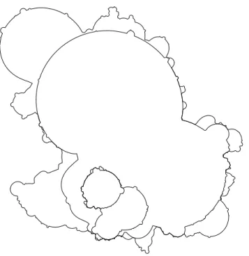
(See Figure 1.1 for an illustration.) Then, we letr→0, and hope that the process, using the increasing setIr(t)of arrivals, will converge to a process(D^z_t,t≥0), the connected component ofzat timet. Moreover, using conformal invariance, we can try to define the process targeted at all pointsz∈Usimultaneously: as long as D_t^z=D^w_t , the processes targeted towardsz andwcoincide, and after the disconnection time they continue independently. Our first result says that this envisioned procedure actually works, but only forκ∈[0,4):

Theorem 1.1. For κ∈[0,4), there exists a growth process (Dt,t≥0) = (D^z_t,t≥0,z∈U) ofSLE_κ excursions, targeted at all points, with the property that(Dt,t≥0)and(ϕ(Dt),t≥0)have the same law (with no time-change) for all M¨obius transformationsϕ ofU. We will abbreviate this Conformal Growth of Excursions byCGEκ.

Maybe disappointingly, CGEκdoes not produce considerable extra fractalness, beyond what is already inherent in the SLEκarcs, which have dimension 1+κ/8 [Bef08]:

1

arXiv:1601.05713v1 [math.PR] 21 Jan 2016

1 Introduction 2

Fig. 1.1: Four stages (75, 150, 300, 500 arcs) of CGE_κ=0, growing towards ∞(that is, the process tar- geted at 0, inverted through the circle for better visibility), with some positive cutoff for the sizes of the SLE₀arcs, which are just semicircles.

Theorem 1.2. Fixκ∈[0,4). Suppose that(D_t⁰,t≥0)isCGE_κ targeted at the origin. DefineΓto be the closure of the union∪_t≥0∂D⁰_t. Then, almost surely,

dim(Γ) =1+κ/8.

Consider now the conformal radius ofD^z_t seen fromz, denoted by CR(z;D_t^z). We can derive the asymptotic decay of the conformal radius. Forλ ∈R, define the Laplace exponent

Λκ(λ) =logE

hCR(z;D^z₁)^−λi .

As we will see,Λ_κ(λ)is finite whenλ<1−κ/8, and we have almost surely that

t→∞lim

−log CR(z;D^zt)

t =Λ⁰_κ(0)∈(0,∞). (1.1)

From (1.1), we know that typically the conformal radius CR(z;D_t^z)decays like exp(−tΛ⁰_κ(0)). We are also inter- ested in those pointszwhere CR(z;D_t^z)decays in an abnormal way. Define, forα ≥0, the random set

Θ(α) =

z∈U: lim

t→∞

−log CR(z;D_t^z)

t =α

. (1.2)

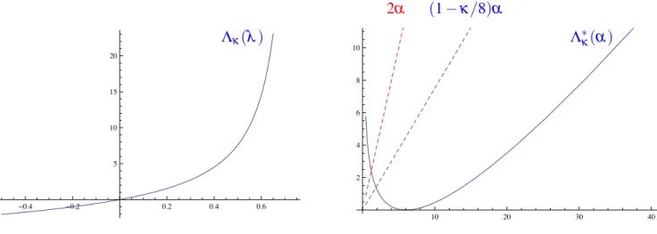
Clearly, whenα 6=Λ⁰_κ(0), the points in the setΘ(α)have an abnormal decaying rate of CR(z;D^zt). The Hausdorff dimension ofΘ(α)can be estimated throughFenchel-Legendre transformofΛ_κ. The Fenchel-Legendre transform ofΛ_κis defined by, forα ∈R,

Λ^∗_κ(α) =sup

λ∈R

(λ α−Λκ(λ)).

1 Introduction 3

!0.4 !0.2 0.2 0.4 0.6

5 10 15 20

10 20 30 40

2 4 6 8

Λ_κ(λ) 10 Λ^∗_κ(α)

2α (1−κ/8)α

Fig. 1.2: Withκ=2, numerical approximations ofΛκ(λ), blowing up atλ =1−κ/8, and its Fenchel- Legendre transformΛ^∗_κ(λ), with an asymptotic slope 1−κ/8.

Theorem 1.3. Define

αmin=sup{α>0 : 2α−Λ^∗_κ(α)≤0}. (1.3) We have almost surely,

(dim(Θ(α))≤2−Λ^∗_κ(α)/α, α ≥αmin; Θ(α) =/0, α <αmin.

The CGE_κ process(Dt,t≥0) targeted at all points naturally yields a fragmentation process of the unit disk, raising interesting questions. First of all, for anyz,w∈U, we can defineT(z,w)to be the first timetsuch thatz,w are not in the same connected component of D_t. We callT(z,w) the disconnection time, for which we have the following estimate:

Theorem 1.4. Fixκ∈[0,4)and letΛκ(λ)be the Laplace exponent defined in (3.10). Let z,w∈Ube distinct and T(z,w) be the disconnection time ofCGE_κ targeted at all points. Then there exists a constant C∈(0,∞)(only depending onκ) such that

E[T(z,w)]−G_U(z,w)/Λ⁰_κ(0) ≤C, where G_Uis Green’s function of the unit disc.

Based on the fragmentation process, we can also construct random fields on the unit disk:

Theorem 1.5. Fixκ ∈[0,4)andδ >0. Suppose thatνis aσ-finite measure supported in[0,∞)with finite mean and unit second moment:

¯ m:=

Z

xν[dx]<∞, Z

x²ν[dx] =1.

Suppose that(Dt,t≥0)isCGEκ targeted at all points, generated fromΓ, the collection ofSLEκ excursions. For each z∈U, denote by D^z_t the connected component of Dt that contains z. GivenΓ, let(σγ)γ∈Γ be i.i.d. weights sampled fromν. Define, for each z∈U, t≥0,

ht(z) =

∑

γ∈Γ

σγ1{γcontributes to D^z_t}−tm.¯ Then we have the following:

2 Preliminaries 4

(1) There exists an H_loc^−2−δ(U)-valued random variable h such that ht→h as t→∞almost surely in H_loc^−2−δ(U).

Moreover, for any f,g∈C^∞_c(U), the covariance betweenhh,fiandhh,giis given by E[hh,fihh,gi] =

ZZ

U×U

f(z)g(w)E[T(z,w)]dzdw, where T(z,w)is the disconnection time ofCGEκ.

(2) The limiting distribution h is almost surely determined byΓand(σγ)γ∈Γ.

(3) The limiting distribution is conformal invariant: letϕbe any M¨obius transformation ofU, and leth be the˜ limiting distribution in H_loc^−2−δ(U)associated withΓ˜ := (γ˜=ϕ(γ),γ ∈Γ)and(σ_ϕ⁻¹_(γ)˜), thenh˜ =h◦ϕ⁻¹ almost surely.

Finally, let us discuss the most obvious question: in what discrete models can one find a structure that has our CGEκas a scaling limit? The full conformal invariance of the process targeted at all points suggests that probably one should look for structures that can be defined not only as growth processes, but also as static objects, similar to the Conformal Loop Ensembles CLE_κ [SW12, WW13, MWW13]; note however that CLE_κ exists for a different subset of κ values: for κ ∈(8/3,4]if the loops are simple, and for κ ∈(8/3,8) in general. Also, from such a discrete static point of view, it would seem to be an important property that the order of attaching the SLE_κ arcs should not matter, and such a commutation relation holds only forκ=2 [KL07]. Therefore, a good candidate for a suitable discrete model isWilson’s algorithm[Wil96], which generates a Uniform Spanning Tree from iteratively adding Loop-Erased Random Walk trajectories, which converge to SLE₂arcs [Sch00, LSW04]. Another discrete model that has many features similar to our CGE_κcould be the construction of acritical percolationconfiguration [Smi01, CN06, Wer07] from the collection of outermost crossings, viewed from an inner point. However, these crossings converge not to SLE_8/3, but different SLE_8/3(ρ)arcs [LSW03, Wer05], hence we do not have an exact correspondence.

Overview of the paper.In Section 2, we define the boundary Poisson kernel and the SLEκand SLEκ(ρ)processes, prove an overshoot estimate for subordinators, and recall a sufficient condition for the convergence of random fields in the sense of distributions.

In Section 3, we prove Theorem 1.1: we construct the growth process forκ<4, prove that it is conformally invariant, and show that it does not exist forκ≥4. The proofs are based on known estimates on the probability that chordal SLE_κcomes close to a point on the boundary or inside the domain, and on conformal martingales related to these questions, describing the Laplace transform of the capacity of an SLEκarc. We also prove Theorem 1.3 on the dimension of points with abnormal decay, using Large Deviations theory.

In Section 4, we give estimates on the disconnection time, proving Theorem 1.4 in particular. Here a key ingre- dient is the innocent-looking Lemma 4.1, saying that the process leaves the boundary∂Uin finite time with positive probability. We also prove Theorem 1.2 on the dimension being 1+κ/8, where the full conformal invariance of the process targeted at all points is of immense help. Finally, we prove Theorem 1.5, constructing the conformally invariant random fields.

We end the paper with three open problems in Section 5.

Acknowledgments. We are indebted to Itai Benjamini for suggesting the model back in 2006, and to Oded Schramm for his insights at the beginning of this project. We also thank St´ephane Benoist, Tom Ellis, Adrien Kas- sel, Gregory Lawler and Wendelin Werner for helpful discussions. G. Pete is partially supported by the Hungarian National Science Fund OTKA grant K109684, and by the MTA R´enyi Institute “Lend¨ulet” Limits of Structures Research Group. H. Wu is supported by the NCCR/SwissMAP, the ERC AG COMPASP, and the Swiss NSF.

2 Preliminaries

Notation.

B(z,r) ={w∈C:|z−w|<r}, U=B(0,1); H={w∈C:ℑw>0}.

2 Preliminaries 5

2.1 Green function and Poisson kernel

Letη(z,·;t)denote the law of 2D Brownian motion(Bs,0≤s≤t)starting fromz. We can write η(z,·;t) =

Z

C

η(z,w;t)dw,

wheredwdenotes the area measure andη(z,w;t)is a measure on continuous curve fromztow. Defineη(z,w) = R_∞

0 η(z,w;t)dt. This is an infinite σ-finite measure. If Dis a domain andz,w∈D, defineηD(z,w)to beη(z,w) restricted to curves stayed inD. Ifz6=wandDis a domain such that a Brownian motion inDeventually exitsD, then the total mass|ηD(z,w)|is finite and we define theGreen function

GD(z,w) =π|η_D(z,w)|.

In particular, whenD=Uandz,w∈U, we have

G_U(z,w) =log

1−zw¯ z−w

.

Just like planar Brownian motion, the Green function is also conformally invariant: ifϕ:D−→ϕ(D)is a conformal map andz,w∈D, then we have

G_ϕ(D)(ϕ(z),ϕ(w)) =GD(z,w). (2.1)

Suppose thatDis a connected domain with piecewise analytic boundary. LetBbe a Brownian motion starting fromz∈Dand stopped at the first exit timeτD:=inf{t:B_t6∈D}. Denote byηD(z,∂D)the law of(Bt,0≤t≤τD).

We can write

ηD(z,∂D) = Z

∂D

ηD(z,w)dw,

wheredwis the length measure on∂DandηD(z,w)is a measure on continuous curves fromztow. The measure ηD(z,w) can be viewed as a measure on Brownian paths starting fromzand restricted to to exit Datw. Define Poisson kernel H_D(z,w)to be the total mass ofηD(z,w).

Suppose thatz,ware distinct boundary points. Define the measure on Brownian paths fromztowinDto be ηD(z,w) =lim

ε→0

1

εηD(z+εnz,w),

wherenzis the inward normal atz. The measureηD(z,w)is called Brownian excursion measure. Define theboundary Poisson kernel HD(z,w)to be the total mass ofηD(z,w). From the conformal invariance of Brownian motion, we can derive the conformal covariance of the boundary Poisson kernel (see [Law05, Proposition 5.5]): Suppose that ϕ:D−→ϕ(D)is a conformal map andz,w∈∂Dandϕ(z),ϕ(w)∈∂ ϕ(D)are analytic boundary points, then

|ϕ⁰(z)ϕ⁰(w)|H_ϕ(D)(ϕ(z),ϕ(w)) =H_D(z,w). (2.2) Moreover, ifD=Uandz,w∈∂U, we have

H_U(z,w) = 1 π|z−w|². In particular, ifθ=arg(z/w)∈[0,2π), we have

H_U(z,w) = 1

4πsin²(θ/2). (2.3)

2 Preliminaries 6

2.2 Chordal and radial SLE

In this section, we review briefly the chordal and radial SLE_κ(ρ)processes and refer the reader to [Wer04] and [Law05] for a detailed introduction. Thechordal Loewner chainwith a continuous driving functionW:[0,∞)→R is the solution for the following ODE: forz∈H,

∂tgt(z) = 2

g_t(z)−W_t, g₀(z) =z.

This solution is well-defined up to the swallowing time T(z):=inf

t: inf

s∈[0,t]|g_s(z)−W_s|>0 .

Fort≥0, defineKt :={z∈H:T(z)≤t}, thengt(·) is the unique conformal map fromH\Kt onto Hwith the expansiong_t(z) =z+2t/z+o(1/z)asz→∞.

Chordal SLE_κ is the chordal Loewner chain with driving functionW =√

κB whereBis a one-dimensional Brownian motion. Forκ ∈[0,4], the SLEκ process is almost surely a continuous simple curve inH from 0 to

∞. Supposeγis an SLE_κ curve inHfrom 0 to∞, then it is conformal invariant: for anyc>0, the curvecγ has the same law asγ(up to time change). Therefore, we could define chordal SLE in any simply connected domain.

Suppose thatDis a simply connected domain andx,y∈∂Dare distinct boundary points. Define SLEκ inDfrom xtoyto be the image of SLE_κinHfrom 0 to∞under any conformal map fromHontoDsending the pair(0,∞) to(x,y).

Chordal SLEκ is reversible: suppose that γ is an SLEκ inDfromxtoy, then the time-reversal of γ has the same law as an SLE_κ inDfromytox. Thus, we also call SLE_κ inDfromxtoyas SLE_κinDwith two end points (x,y).

Theradial Loewner chainwith a continuous driving functionW:[0,∞)→∂Uis the solution for the following ODE: forz∈U,

∂tg_t(z) =g_t(z)W_t+g_t(z)

Wt−gt(z), g₀(z) =z.

This solution is well-defined up to the swallowing time T(z):=inf

t: inf

s∈[0,t]|g_s(z)−W_s|>0 .

Fort≥0, define Kt :={z∈U:T(z)≤t}, thengt(·)is the unique conformal map from U\Kt ontoU with the normalization: g_t(0) =0,g⁰_t(0)>0.

RadialSLE_κ is the radial Loewner chain with driving functionW=exp(i√

κB)whereBis a one-dimensional Brownian motion. Forκ∈[0,8), radial SLEκis almost surely a continuous curve inUfrom 1 to the origin.Radial SLE_κ(ρ) withW₀=x∈∂Uand force pointV₀=y∈∂U is the radial Loewner chain with driving functionW solving the following SDEs:

dWt=i√ κBt−

κ 2Wt+ρ

2Wt

Wt+Vt

W_t−V_t

dt, W₀=x;

dV_t=V_tW_t+Vt

W_t−V_tdt, V₀=y.

The system has a unique solution up to the collision time

T :=inf{t:Wt =Vt}.

We focus on the weightρ=κ−6 for the following reason: chordal SLEκinUfromxtoyhas the same law as radial SLEκ(κ−6)with starting pointW₀=xand force pointV₀=y; see [SW05]. Fixκ ∈[0,8)andρ=κ−6.

Defineθt =arg(Wt)−arg(Vt)∈(0,2π), then by Itˆo’s formula, the processθt satisfies the SDE:

dθt=√

κdBt+κ−4

2 cot(θt/2)dt. (2.4)

2 Preliminaries 7

The collision timeT is also the first time thatθt hits 0 or 2π. Moreover, whenκ∈[0,8), we haveE[T]<∞.

Suppose thatDis a proper simply connected domain. Theconformal radiusofDseen fromz∈Dis|ϕ⁰(z)|⁻¹ whereϕis any conformal map fromDontoUsendingzto the origin. We denote this conformal radius by CR(z;D).

Define the inradius

inrad(z;D):= inf

w∈C\D|z−w|.

By Koebe’s one quarter theorem and the Schwarz lemma [Law05, Theorem 3.17, Lemma 2.1], we have that

inrad(z;D)≤CR(z;D)≤4 inrad(z;D). (2.5)

For any compact subsetK⊂U, letDbe the connected component ofU\Kthat containsz. Define thecapacityof Kseen fromzto be

cap(z;K) =−log CR(z;D).

Whenzis the origin, we simply denote CR(0;D)and cap(0;K)by CR(D)and cap(K)respectively. One can check that the radial Loewner chain is parameterized by capacity seen from the origin.

2.3 Overshoot estimate for subordinators

Suppose that (X(t),t ≥0) is a right-continuous increasing process starting from 0 and taking values in [0,∞).

We callX a subordinator if it has independent homogeneous increments on [0,∞). The Laplace transform of a subordinator has a nice expression: for t>0 and λ ≥0, we have E[exp(λX(t))] =exp(−tΦ(λ)), where Φ: [0,∞)→[0,∞). There exist a unique constantd≥0 and a unique measureΠon(0,∞), which is called the L´evy measure ofX, with^R(1∧x)Π(dx)<∞such that, forλ ≥0,

Φ(λ) =dλ+ Z

(1−e^−λx)Π(dx).

Moreover, one has almost surely, fort>0,

X(t) =dt+

∑

s≤t

∆s,

where(∆s,s≥0)is a Poisson point process with intensity Π. (More precisely, we have a Poisson point process {(∆j,sj): j∈J}with intensityΠ⊗Lebesgueon (0,∞)×[0,∞), the second coordinate being time, whereJ is a countable set, and we let∆s:=∆j whens=sj, while∆s:=0 otherwise.) Define the tail of the L´evy measure:

Π(x) =Π((x,∞)).

We introduce the inverse ofX: forx>0,

Lx=inf{t:X(t)>x}, and the processes of first-passage and last-passage ofX: forx>0,

D_x=X(Lx), G_x=X(Lx−).

A subordinator is a transient Markov process, its potential measureU(dx)is called the renewal measure. It is defined as, for any nonnegative measurable function f,

Z _∞

0

f(x)U(dx) =E Z _∞

0

f(X(t))dt

.

Proposition 2.1. For every real numbers a,b,x such that0≤a<x≤a+b, we have that P[Gx∈da,Dx−Gx∈db] =U(da)Π(db).

2 Preliminaries 8

Proof. [Ber99, Lemma 1.10].

Proposition 2.2. Suppose that X is a subordinator with L´evy measureΠsatisfying Z

(e^λ0x−1)Π(dx)<∞, for someλ0>0.

Then there exists a positive finite constant C (depending onΠandλ₀) such that P[Dx−x≥y]≤Ce^−λ0y, for all x≥0,y≥0.

Proof. When y∈[0,1], we could takeC≥e^λ0. Thus we can supposey≥1. We divide the event {D_x−x≥y}

according to the values ofGx. For everyk∈N, define

Ek= [Gx≤x−k,Dx≥x+y].

By Proposition 2.1, we have that

P[Ek]≤Π(k+y)

≤ Z

u≥k+ye^λ0ue^−λ0(k+y)Π(du)

≤e^−λ0(k+y) Z

u≥1

e^λ0uΠ(du).

Thus

P[Dx−x≥y]≤

∑

k≥0

P[Ek]≤e^−λ0y R

u≥1e^λ0uΠ(du) 1−e^−λ0 . So we can take

C=e^λ0∨ R

u≥1e^λ0uΠ(du) 1−e^−λ0 .

Remark 2.3. In the literature, people usually consider right-continuous subordinators. Whereas, the conclusions in this section also hold for left-continuous subordinators. Note that if X is a left-continuous subordinator, then X can be written as, for t>0,

X(t) =dt+

∑

s<t

∆s,

where(∆s,s≥0)is a Poisson point process. Therefore, the proofs in this section can be modified for left-continuous subordinators without difficulty. In the later part of our paper, we will apply conclusions in this section for left- continuous subordinators.

2.4 Convergence of distributions

In this subsection, we give an overview of the convergence of distributions. We refer the reader to [Tao10, Section 1.13] for a more detailed introduction to the space of distributions and to [MWW13, Section 5] for the proof of the convergence result of distributions that we will need.

Fix a positive integerd. TheSchwartz space S(R^d)is defined to be the space of smooth functions f:R^d−→C such that all derivatives are rapidly decreasing, i.e.,|x|ⁿk∇^jf(x)kis bounded for all non-negative integersnand j where we view∇^jf(x)as ad^j-dimensional vector. We equipS(R^d)with the topology generated by the family of seminormskfk_n,j:=sup_x∈Rd|x|ⁿk∇^jf(x)kforn,j≥0.

The space S(R^d)^∗ of tempered distributions is defined to be the space of continuous linear functionals on S(R^d). We write the evaluation ofh∈S(R^d)^∗on f∈S(R^d)with the notationhh,fi. Forh∈S(R^d)^∗, we say that

3 Construction of the growth processCGEκ 9

h is supported in a closed setK ifhh,fi=0 for all f ∈S(R^d)that vanish on an open neighborhood of K. The support ofhis the intersection of allKthathis supported on. Forh∈S(R^d)^∗and f ∈C_c^∞(R^d), define the product h f ∈S(R^d)^∗byhh f,gi=hh,f gi¯ for allg∈S(R^d).

For f ∈S(R^d), the Fourier transform and its conjugate are defined by F(f)(ξ) =

Z

e^−2πix·ξf(x)dx, F^∗(f)(ξ) = Z

e^2πix·ξf(x)dx, ∀ξ ∈R^d.

Note that f∈S(R^d)impliesF(f)∈S(R^d). We may define the Fourier transform of a tempered distributionhby hF(h),fi:=hh,F^∗(f)ifor all f∈S(R^d). We also denoteF(h)by ˆh.

For anys∈R, define theSobolev space H^s(R^d)to be the space of all tempered distributionshsuch that the distributionhξi^sh(ξˆ )lies inL²(R^d)wherehξi:= (1+|ξ|²)^1/2. The spaceH^s(R^d)is a Hilbert space with the inner product

hf,gi_H^s_(R^d₎:=

Z

hξi^2sfˆ(ξ)g(ξˆ )dξ.

LetD⊂R^d be an open set. Forh∈C_c^∞(R^d)^∗, we say thath∈H_loc^s (D)ifh f ∈H^s(D)for all f∈C_c^∞(D). We equipH_loc^s (D)with a topology generated by the seminorms kf· k_Hs(R^d), which implies that hn→hinH_loc^s (D)if and only ifhh_n,fi → hh,fiinH^s(R^d)for all f ∈C_c^∞(D).

Proposition 2.4. Let D⊂R^dbe an open set andδ>0. Suppose that(hn)n∈Nis a sequence of random measurable functions defined on D satisfying the following conditions: for every compact K⊂D,

(1) for all n≥1, we have

Z

KE[|hn(z)|²]dz<∞;

(2) there exists a summable sequence(an)n∈Nof positive reals such that, for all n≥1, we have ZZ

K×K

|E[(h_n+1(z)−h_n(z))(h_n+1(w)−h_n(w))]|dzdw≤a³_n.

Then there exists a random element h∈H_loc^−d−δ(D)supported on the closure of D such that almost surely hn→h in H_loc^−d−δ(D).

Proof. [MWW13, Proposition 5.1].

3 Construction of the growth process CGE

3.1 The Poisson point process of SLE excursions

LetH_U(x,y)be the boundary Poisson kernel for the unit discUwith distinct boundary pointsx,y∈Uas introduced in Section 2.1. Denote byµ^#

U,κ(x,y)the law of chordal SLE_κ inUwith two end pointsx,y. Forκ∈[0,8), define the SLE_κ excursion measureto be

µ_U,κ= Z Z

dxdyH_U(x,y)µ_U,κ^# (x,y), (3.1)

where dx,dy are length measures on ∂U. Note that µ_U,κ is an infinite σ-finite measure. From the conformal invariance of SLE and the conformal covariance of boundary Poisson kernel (2.2), we can derive the conformal invariance of SLE excursion measure.

Proposition 3.1. TheSLEexcursion measureµ_U,κis conformal invariant: for any M¨obius transformationϕofU, we have

ϕ◦µ_U,κ=µ_U,κ, whereϕ◦µ[A]:=µ[γ:ϕ(γ)∈A].

3 Construction of the growth processCGEκ 10

We will construct a growth process from a Poisson point process of SLE excursions. The construction is not surprising if one is familiar with [SW12] and [WW13]. To be self-contained, we briefly explain the construction.

Let(γt,t≥0)be a Poisson point process with intensityµ_U,κ. More precisely, let((γj,tj),j∈J)be a Poisson point process with intensityµ_U,κ⊗[0,∞), and then arrange the excursionsγj according totj: denote the excursionγj by γt ift=t_jandγt is empty set if there is not_j that equalst. There are only countably many excursions in(γt,t≥0) that are not empty set. Forκ∈[0,8), with probability one there is noγt passing through the origin. For eachtsuch thatγt is not the empty set, the curveγt separatesUinto two connected components, and we denote byU_t⁰the one that contains the origin. Let f_tbe the conformal map fromU_t⁰ontoUnormalized at the origin: f_t(0) =0,f_t⁰(0)>0.

Fort>0, define the accumulated capacity to be

Xt =

∑

s<t

cap(γs).

Proposition 3.2. For t>0, the accumulated capacity Xt is almost surely finite if and only ifκ∈[0,4).

We will complete the proof of Proposition 3.2 in Section 3.3. Assuming Proposition 3.2, we can now construct the growth process forκ∈[0,4). For any fixedT>0 andr>0, lett₁(r)<t₂(r)<· · ·<tj(r)be the timestbefore T at which the distance between the two end points ofγt is at leastr. Define

Ψ^r_T =f_tj(r)◦ · · · ◦f_t1(r).

The mapΨ^r_T is a conformal map from some subset ofUontoU. By Proposition 3.2, we know thatXT<∞almost surely whenκ ∈[0,4). Then the conformal mapΨ^r_T converges almost surely in the Carath´eodory topology seen from the origin, asr→0; see [SW12, Section 4.3, Stability of Loewner chains]. Define

D⁰_t :=Ψ_t⁻¹(U),t≥0 .

This is a decreasing sequence of simply connected domains containing the origin, and we call itthe growth process CGE_κ ofSLEexcursions targeted at the origin. By the conformal invariance of the SLE excursion measure, we can derive the conformal invariance of CGEκ.

Lemma 3.3. Forκ∈[0,4), the law of the growth process(D_t⁰,t≥0)is conformally invariant under any M¨obius transformationϕofUthat preserves the origin.

Proof. Let(γˆt,t≥0)be a Poisson point process with intensityµ_U,κ, and define ˆft and ˆΨt for eachtas described above, and denote by(Dˆ⁰_t,t≥0)the corresponding growth process targeted at the origin.

By Proposition 3.1, we know that the process(γt :=ϕ(γˆt),t≥0)is also a Poisson point process with intensity µ_U,κ. Define ft andΨt for eacht, and denote by(D⁰_t,t≥0)be the corresponding growth process targeted at the origin. It is clear that

f_t =ϕ◦fˆ_t◦ϕ⁻¹, Ψt =◦_s<tf_s=ϕ◦Ψˆt◦ϕ⁻¹.

Since(γt,t≥0)has the same law as(γˆt,t≥0), the process(D_t⁰=ϕ(Dˆ_t⁰),t≥0)has the same law as(Dˆ_t⁰,t≥0)as desired.

We can construct CGE_κ targeted at anyz∈Uin the same way as above, except that we choose to normalize at zinstead of normalizing at the origin. Another way to describe CGEκ targeted atzwould be(ϕ(D⁰_t),t≥0)where ϕis any M¨obius transformation ofUthat sends the origin toz. By Lemma 3.3, the choice ofϕ does not affect the law of(ϕ(D⁰_t),t≥0), thus CGE_κ targeted atzis well-defined.

Now we will describe the relation between two growth processes targeted at distinct points z,w∈U. Let (D^z_t,t≥0) (resp. (D^w_t ,t≥0)) be CGE_κ processes targeted at z (resp. targeted atw), and define T(z,w) (resp.

T(w,z)) to be the first timetthatw6∈D^z_t (resp. z6∈D_t^w). We callT(z,w)the disconnection time. The interesting property of these growth processes is that the two processes have the same law up to the disconnection time.

Proposition 3.4. For κ ∈[0,4), and for any z,w∈U, the law of (D_t^z,t <T(z,w)) is the same as the law of (D^w_t ,t<T(w,z)).

3 Construction of the growth processCGEκ 11

Proof. Recall a classical result about Poisson point processes (see [Ber96, Section 0.5]): Let(at,t≥0)be a Poisson point process with some intensityν(defined in some metric spaceA). LetFt−=σ(as,s<t). If(Φt,t≥0)is a process (with values on functions ofAtoA) such that for anyt>0,Φt isFt−-measurable, and thatΦt preserves ν, then(Φt(at),t≥0)is still a Poisson point process with intensityν.

Let(γˆt,t≥0)be a Poisson point process with intensityµ_U,κand defineFt−=σ(γˆs,s<t), let ˆf_t^zand ˆΨ_t^zbe the conformal maps as described above normalized atz. Let(Dˆ^z_t,t≥0)be the corresponding growth process targeted atzand ˆT(z,w)be the first timet thatw6∈Dˆ_t^z. For eacht<Tˆ(z,w), the domain ˆD^z_t containsw, and letGt be the conformal map from ˆD^z_t ontoUnormalized atw:G_t(w) =wandG_t⁰(w)>0.

For eacht<Tˆ(z,w), define ϕt =Gt◦(Ψˆ^z_t)⁻¹. Fort=Tˆ(z,w), defineϕt =lims↑tϕs. Fort>Tˆ(z,w), define ϕt to be identity map. Note that ˆΨt^z=◦_s<tfˆ_s^zand thus ˆΨ^zt isFt−-measurable. Therefore, for allt>0,ϕt isFt−- measurable. By Proposition 3.1 and the classical result of Poisson point process recalled at the beginning of the proof, we know that (γt :=ϕt(γˆt),t≥0) is also a Poisson point process with intensity µ_U,κ. For(γt,t≥0), let (D^w_t ,t≥0)be the corresponding growth process targeted atwand letT(w,z)be the first timetthatz6∈D^w_t . By the construction, we have that

D_t^w=Dˆ^z_t, for allt<T(w,z).

Hence, in this coupling, we haveT(w,z)≤Tˆ(z,w). By symmetry, we have thatT(w,z) =Tˆ(z,w)almost surely. In particular, this coupling implies that the two disconnection times have the same law, and the two growth processes (D^z_t,t≥0)and(D_t^w,t≥0)have the same law up to the disconnection time.

Proposition 3.4 tells that, for any z,w∈U, it is possible to couple the two growth processes targeted atzand wrespectively to be identical up to the first time at which the pointsz,ware disconnected. Hence, it is possible to couple the growth processes(D^z_t,t≥0) for allz in a fixed countable dense subset ofUsimultaneously in such a way that for any two pointszandw, the above statement holds.

For such a coupling, we get a Markov process on domains(Dt,t≥0): Att=0, the domain isU, and at time t>0, it is the union of all the disjoint open subsets corresponding to the growth process targeted at all pointsz at timet. We call this Markov processthe conformal growth process ofSLEexcursions targeted at all points, or CGEκ. By construction, it is naturally conformal invariant. This completes the proof of Theorem 1.1.

In Subsections 3.2 and 3.3, we will calculate the Laplace transform of the accumulated capacity and complete the proof of Proposition 3.2.

3.2 The Laplace transform of the capacity of chordal SLE

In this section, we will calculate the Laplace transform of the capacity of chordal SLEκ inU. To this end, we need to recall some basic facts about hypergeometric functions. The hypergeometric function is defined for|z|<1 by the power series

φ(a,b;c;z) =

∞ n=0

∑

(a)n(b)n

(c)nn! zⁿ, (3.2)

where(q)nis the Pochhammer symbol defined by (q)n=

(1, n=0;

q(q+1)· · ·(q+n−1), n≥1.

The function in (3.2) is only well-defined forc6∈ {0,−1,−2,−3...}. The hypergeometric function is a solution of Euler’s hypergeometric differential equation

−abφ+ (c−(a+b+1)z)φ⁰+z(1−z)φ⁰⁰=0. (3.3) Note that, whenc6∈Z, the following function is also a solution to Equation (3.3):

z^1−cφ(1+a−c,1+b−c; 2−c;z).

3 Construction of the growth processCGEκ 12

Proposition 3.5. Fixκ∈[0,8)andλ ∈(0,1−κ/8). Suppose thatγ=γ^θ is a chordalSLEκinUfrom x∈∂Uto y∈∂U, whereθ=arg(x)−arg(y). Define three constants

a=1−4 κ+

s

1−4 κ

2

+8λ

κ , b=1−4 κ−

s

1−4 κ

2

+8λ

κ , c=3 2−4

κ. Assume that c6∈Z. Define two functions f and g: for u∈[0,1],

f(u) =φ(a,b;c;u), g(u) =u^1−cφ(1+a−c,1+b−c; 2−c;u).

Then, we have

E[exp(λcap(γ^θ))] =f(u) +(1−f(1))

g(1) g(u), (3.4)

where u=sin²(θ/4).

Proof. First, let us check the values of the functions f andg at the end pointsu=0 oru=1. Sinceκ∈[0,8), λ ∈(0,1−κ/8)andc6∈Z, we have that

a∈(0,1), b∈(1−8/κ,0), c∈(−∞,1)\Z.

Combining with [Bat53, Page 104, Equation (46)], we have that (denoting byΓthe Gamma function)

f(0) =1, f(1) =Γ(c)Γ(c−a−b) Γ(c−a)Γ(c−b)=

cos

π q

1−⁴

κ

2

+^8λ_κ

cos π 1−_κ⁴ ∈[−1,1);

g(0) =0, g(1) = Γ(2−c)Γ(1−c)

Γ(1−a)Γ(1−b) ∈(0,∞).

Second, assuming the same notation as in Subsection 2.2, we know thatγhas the same law as radial SLEκ(κ− 6)with(W₀,V₀) = (x,y). Letθt =arg(Wt)−arg(Vt), we will argue thate^λtf(sin²(θt/4))ande^λtg(sin²(θt/4))are martingales up to the collision timeT. Suppose thatF is an analytic function defined on(0,1). By the SDE (2.4) and Itˆo’s formula, we know thate^λtF(sin²(θt/4))is a local martingale if and only if

λF(u) +3κ−8

16 (1−2u)F⁰(u) +κ

8u(1−u)F⁰⁰(u) =0.

Since fandgare solutions to this ODE, we know thate^λtf(sin²(θt/4))ande^λtg(sin²(θt/4))are local martingales.

Since f andgare finite at end points u=0 andu=1, and the collision timeT has finite expectation, we may conclude that the processese^λtf(sin²(θt/4))ande^λtg(sin²(θt/4))are martingales up toT.

Finally, we derive Equation (3.4). Sincee^λtf(sin²(θt/4))ande^λtg(sin²(θt/4))are martingales up toT which has finite expectation, Optional Stopping Theorem gives

E

exp(λT)1{θ_T=0}

+f(1)E

exp(λT)1{θ_T=2π}

= f(u);

g(1)E

exp(λT)1_{θT=2π}

=g(u).

These give Equation (3.4) by noting that cap(γ) =T.

Remark 3.6. The martingale e^λtf(sin²(θt/4))in the proof of Proposition 3.5 was studied in [SSW09].

Remark 3.7. Forκ∈[0,8), suppose thatγ is a chordalSLEκinUwith distinct end points x,y∈∂U. Forλ∈R, define

F(κ,λ) =E[exp(λcap(γ))].

On the one hand, by Proposition 3.5, we see that when c=3/2−4/κ6∈Zandλ <1−κ/8, the quantity F(κ,λ) is finite. On the other hand, we know that F(κ,λ)is continuous in(κ,λ)(for the continuity inκ; see for instance [KS12, Theorem 1.10]). Therefore, the quantity F(κ,λ)is finite for allκ∈[0,8)andλ<1−κ/8.

3 Construction of the growth processCGEκ 13

Since the boundary Poisson kernelH_U(x,y)blows up whenθ=arg(x)−arg(y)is small, in order to understand the excursion measureµ_U,κ, it will be important for us how the capacity cap(γ^θ)behaves asθ→0.

Proposition 3.8. Fixκ∈[0,8)such that c(κ) =³₂−⁴

κ 6∈Z, andλ∈(0,1−κ/8). Asθ→0, or equivalently, u→0, the Laplace transform of the capacity satisfies

E

exp(λcap(γ^θ))−1

u^1−c θ^2(1−c) if 8/3<κ<8,

u θ² if 0<κ<8/3, c6∈Z−, (3.5) with the constant factors implicit independing onκandλ. Quite similarly, the expectation itself satisfies

E

cap(γ^θ)







u^1−c θ^2(1−c) if 8/3<κ<8, ulog(1/u) θ²log(1/θ) if κ=8/3,

u θ² if 0≤κ<8/3,

(3.6)

with the constant factors implicit independing onκ.

Proof. For the functions given in Proposition 3.5 for the casec6∈Z, it is easy to check that f(u)−1= f(u)−f(0) decays likeuasu→0 andg(u)decays likeu^1−c asu→0. This gives (3.5), with a phase transition atc=0, that is, atκ=8/3.

To get the expectation (3.6), one possibility would be to take the derivative of the Laplace transformF(κ,λ)at λ=0. However, our formula (3.4) is not particularly simple, hence this task is not obvious. Another approach could be to argue that, for smallθ, it is very likely that cap(γ^θ)is also small, hence exp(λcap(γ^θ))−1 andλcap(γ^θ)are likely to be close to each other, and hence it is not surprising if theu→0 asymptotics of their expectations are the same. However, a large portion of the expectations might come from when cap(γ^θ)is large, hence this argument would also need some extra work. Finally, we have (3.4) and (3.5) only whenc(κ)6∈Z, which is an immediate drawback to start with. Therefore, we give the following separate and direct argument.

Forκ∈(0,8)andθ<r<1/4, it follows immediately from the results of [AK08] that

P[diam(γ^θ)>r](θ/r)^8/κ−1. (3.7) When the diameter is in [r,2r), the capacity is at mostCr². Moreover, if a curveγ^θ going from exp(−iθ/2)to exp(iθ/2)has diameter in[r,2r), and it also separates the center 0 from the point 1−r/2, then its capacity is at leastcr². For SLE_κ from exp(−iθ/2)to exp(iθ/2), conditioned to have diameter in[r,2r), this separating event has a uniformly positive probability, hence (3.7) implies that

E

cap(γ^θ)1{diam(γ^θ)∈[2^kθ,2^k+1θ)}

(2^kθ)²(2^−k)^8/κ−1=θ²(2^k)^3−8/κ. (3.8) Summing this up over dyadic scales from aroundθto around 1/4, we get that

E

cap(γ^θ)1{cap(γ^θ)<1}







θ^8/κ−1 if κ>8/3, θ²log(1/θ) if κ=8/3, θ² if κ<8/3.

Note that the last line holds even forκ=0.

Now, cap(γ^θ)is larger than t≥1 only ifγ^θ comes closer than exp(−t)to 0. The probability of this has an exponential tail by the one-point estimate in the dimension upper bound [RS05, Lemma 6.3, Theorem 8.1], so this part of the probability space does not raise the expectationE[cap(γ^θ)]by more than a factor, and the proof of (3.6) is complete.

3 Construction of the growth processCGEκ 14

3.3 The Laplace transform of the accumulated capacity

Forκ∈[0,8), recall thatµ_U,κis the SLE excursion measure defined in (3.1). Let(γt,t≥0)be a PPP with intensity µ_U,κand define the accumulated capacity in the same way as before:

X_t =

∑

s<t

cap(γs).

By Campbell’s formula, we have that, forλ ∈R, E[exp(λXt)] =exp

t

Z

(e^λcap(γ)−1)µ_U,κ[dγ]

. (3.9)

In particular, the left hand side of (3.9) is finite if and only if the right hand side is finite. We will study the Laplace exponent

Λ_κ(λ):=

Z

(e^λcap(γ)−1)µ_U,κ[dγ] = Z Z

dxdyH_U(x,y)µ_U^#_,κ(x,y)h

e^λcap(γ)−1 i

. (3.10)

Proposition 3.9.

(1) Whenκ∈[0,4), the Laplace exponentΛκ(λ)is finite forλ∈(0,1−κ/8)and infinite forλ ≥1−κ/8. If κ≥4, thenΛ_κ(λ)is infinite for allλ >0.

(2) Whenκ∈[0,4), we have thatE[Xt]<∞for all t. Whenκ≥4, we have thatE[Xt] =∞for all t>0.

Proof. First, we show that Λ_κ(λ) is finite whenκ ∈[0,4), λ ∈(0,1−κ/8), andc :=3/2−4/κ 6∈Z. Note that, in (3.10), the boundary Poisson kernel and the expectationµ_U,κ^# (x,y)

e^λcap(γ)−1

only depend on the angle difference ofx,y. Assuming the same notation as in Proposition 3.5, we see that

Λ_κ(λ) =4π Z _π

0

dθ

4πsin²(θ/2)µ_U,κ^# (1,e^iθ)h

e^λcap(γ)−1 i

(by (2.3))

= Z _π

0

dθ sin²(θ/2)

f(sin²(θ/4))−1+1−f(1)

g(1) g(sin²(θ/4))

(by (3.4))

=1 2

Z _1/2

0

du u^−3/2(1−u)^−3/2

f(u)−1+1−f(1) g(1) g(u)

. (setu=sin²(θ/4))

Using the decay rate (3.5) of Proposition 3.8, the exponentΛ_κ(λ)is finite forλ∈(0,1−κ/8)whenc<1/2 which is to sayκ<4, and infinite for everyλ>0 whenκ≥4.

That is,Λ_κ(λ)is finite forκ∈[0,4)\ {8/3,8/5,8/7, ....}andλ∈(0,1−κ/8). It is infinite whenλ≥1−κ/8, since already the integrand, the right hand side of (3.4), explodes.

To extend this forκ∈ {8/3,8/5,8/7, ....}, the continuity ofκ 7→F^θ(κ,λ)mentioned in Remark 3.7 implies that the singularity in the integrand can be bounded from above by something integrable whenλ <1−κ/8, and from below by something non-integrable whenλ ≥1−κ/8.

For part (2) regardingE[Xt], we can do the analogous calculation, just using the decay rate (3.6) instead of (3.5).

Proof of Proposition 3.2. Whenκ∈[0,4), we proved in Proposition 3.9 thatE[Xt]is finite, and thus the accumu- lated capacityX_t is finite almost surely.

Next, we will argue thatXtdiverges almost surely whent>0,κ≥4. Fork≥1, defineMkto be the number of excursionsγswiths<tsuch that 2^−k≤cap(γs)<2^−k+1. Since(γs,s≥0)is a PPP with intensityµ_U,κ, we know thatM_kis a Poisson random variable with parameter

q_k:=tµ_U,κ[γ: 2^−k≤cap(γ)<2^−k+1].

3 Construction of the growth processCGEκ 15

By part (2) of Proposition 3.9 , we haveE[Xt] =∞forκ≥4, thus

∑

k≥1

2^−kqk≥E[Xt]/2=∞.

Since(Mk,k≥1)are independent Poisson random variables, we have E

"

exp −

∑

k≥1

2^−kMk

!#

=Πk≥1E h

exp

−2^−kMk

i

=Πk≥1exp

−qk

1−e^−2−k

=0.

Therefore, whenκ≥4, we almost surely have

X_t ≥

∑

k≥1

2^−kM_k=∞.

3.4 Extremes of the conformal radii

Fixκ∈[0,4), by Proposition 3.9, we know that the Laplace exponentΛ_κ(λ)is finite for λ ∈(−∞,1−κ/8). In particular, this implies that it is differentiable on(−∞,1−κ/8)(see [DZ10, Lemma 2.2.5]). Moreover, by Strong Law of Large Numbers for subordinators ([Ber96, Page 92]), we have almost surely that

t→∞lim X_t

t =Λ⁰_κ(0)∈(0,∞),

which implies (1.1). To prove Theorem 1.3, we first summarize some basic properties ofΛ_κ(λ)andΛ^∗_κ(x) (see [DZ10, Lemmas 2.2.5, 2.2.20], and our Figure 1.2 in the Introduction):

(1) The Laplace exponentΛ_κ(λ)is convex and smooth on(−∞,1−κ/8).

(2) The Fenchel-Legendre transformΛ^∗_κ(x)is non-negative, convex, and smooth on(0,∞).

(3) We have Λ^∗_κ(x) =0 when x=Λ⁰_κ(0), the function Λ^∗_κ is increasing on(Λ⁰_κ(0),∞) and is decreasing on (0,Λ⁰_κ(0)).

(4) SinceΛκ(λ)→ −∞asλ → −∞, we know that

Λ^∗_κ(0) = +∞, Λ^∗_κ(x)↑+∞asx↓0.

(5) Asx→+∞, we have

x→∞lim Λ^∗_κ(x)

x =1−κ/8.

Recall thatαminis defined through (1.3). From the above properties, we know that 2x−Λ^∗_κ(x) =0 has a unique solution which is equal toαmin∈(0,Λ⁰_κ(0)). We can complete the proof of Theorem 1.3 using the theory of large deviations:

Proof of Theorem 1.3. It suffices to give upper bound forΘ(α)∩B(0,1−δ)for anyδ>0. Fixα≥0 and assume β >α. Forn≥1, letUnbe the collection of open balls with centers ine^−nβZ²∩B(0,1−δ/2)and radius e^−nβ. For each ballU∈Un, denote byz(U)the center ofU. Define, foru⁻<u⁺,

Un(u⁻,u⁺) =







U∈Un:u⁻≤

−log CR

z(U);D^z(U)n

n ≤u⁺





 .

4 Convergence to a limiting field 16

By Cram´er’s theorem (see [DZ10, Theorem 2.2.3]), foru⁻<u⁺, for anyU∈Un, we have P[U∈Un(u⁻,u⁺)] =P

h

u⁻n≤ −log CR

z(U);D^z(U)n

≤u⁺n i

≤exp

−n

inf

u⁻≤u≤u⁺Λ^∗_κ(u) +o(1)

, (3.11)

where theo(1)term tends to zero asn→∞uniformly inU. Define Cm(u⁻,u⁺) =∪_n≥mUn(u⁻,u⁺).

We claim that Cm(α⁻,α⁺) is a cover for Θ(α)∩B(0,1−δ) for any α⁻<α <α⁺ <β and any m≥1. Pick α˜⁻∈(α⁻,α),α˜⁺∈(α,α⁺). For anyz∈Θ(α)∩B(0,1−δ), since lim(−log CR(z;D^z_n))/n=α, we have that, for nlarge enough,

exp(−nα˜⁻)≥CR(z;D^z_n)≥exp(−nα˜⁺).

Letwbe the point ine^−nβZ²that is the closest tozand denote byU the ball inUnwith centerw. Since ˜α⁺<β and by (2.5), we know thatwis contained inD^z_n. Moreover, fornlarge enough, by (2.5) and thatβ >α⁺>α˜⁺>

˜

α⁻>α⁻, we have

CR(w;D^w_n)≥inrad(w;Dn)≥inrad(z;Dn)−e^−nβ≥1

4CR(z;Dn)−e^−nβ≥1

4e^−nα˜+−e^−nβ ≥e^−nα+. CR(w;D^w_n)≤4 inrad(w;D_n)≤4(inrad(z;D_n) +e^−nβ)≤4(CR(z;Dn) +e^−nβ)≤4(e^−nα˜−+e^−nβ)≤e^−nα−. Thereforez∈U∈Un(α⁻,α⁺). This implies thatCm(α⁻,α⁺) is a cover forΘ(α)∩B(0,1−δ). We use these covers to bounds-Hausdorff measure ofΘ(α)∩B(0,1−δ). Form≥1, andα⁻<α <α⁺<β, we have

E[Hs(Θ(α)∩B(0,1−δ))]≤E

"

∑

U∈Cm(α⁻,α⁺)

|diam(U)|^s

#

≤

∑

n≥m

exp(2nβ)×exp(−snβ)×exp

−n

inf

α⁻≤u≤α⁺Λ^∗_κ(u) +o(1)

(By (3.11))

=

∑

n≥m

exp

n

2β−sβ− inf

α⁻≤u≤α⁺Λ^∗_κ(u) +o(1)

Ifs>2−inf_α⁻≤u≤α⁺Λ^∗_κ(u)/β, then (takingm→∞) we haveE[Hs(Θ(α)∩B(0,1−δ))] =0. This implies that 2− inf

α⁻≤u≤α⁺Λ^∗_κ(u)/β ≥dim(Θ(α)), almost surely.

This holds for anyβ >α⁺>α>α⁻, thus by the continuity ofΛ^∗_κ, we have 2−Λ^∗_κ(α)/α≥dim(Θ(α)), almost surely.

Finally, whenα <αmin, we see thatH0(Θ(α)∩B(0,1−δ)) =0 almost surely. This implies thatΘ(α) = /0 almost surely.

4 Convergence to a limiting field

4.1 Estimates on the disconnection time

The following lemma is the key result of this section:

4 Convergence to a limiting field 17

Lemma 4.1. Fixκ ∈[0,4). Let(D⁰_t,t≥0)beCGEκtargeted at the origin. Then there exist constants r₀∈(0,1), p₀∈(0,1)and t₀>0such that

P

D⁰_t0⊂B(0,r₀)

≥p₀.

Proof. Since the closure ofD⁰_t is a compact subset of the unit disc, it is sufficient to show that there exist constants p₀∈(0,1)andt₀>0 such that

P[∂U∩∂D_t⁰₀= /0]≥p₀. (4.1)

First, we argue that there existu,r,δ >0 such that for any arcI⊂∂Uwith length less thanδ, we have

P[I∩∂D⁰_u=/0]≥r. (4.2)

LetJ be the collection of positive-length arcs of∂Uwith both endpoints in{e^iθ :θ∈Q}. Fix any u>0; since

∂D⁰_u∩∂Uis a compact proper subset of∂U, we know that∂U\∂D⁰_uis a union of open arcs, thus

I∈J

∑

P[I∩∂D⁰_u=/0]>0.

Thus there existsI₀∈Jsuch thatδ:=|I₀|>0 and

r:=P[I₀∩∂D⁰_u=/0]>0.

SinceD⁰_uis rotation invariant, we obtain (4.2).

For ε>0, defineE(ε)to be the collection of excursionsγ inUwith the following property: ifx,y∈∂Uare the two endpoints ofγ, we require that the arc-length fromxtoybe less than ε and that γ disconnect the origin from the arc fromytox. Denote byE(γ)the event thatγ has this property. A standard SLE calculation (see, for instance, [Sch01]) shows that there is a universal constantC<∞such that

q(ε):=µ[E(ε)] = Z Z

|x−y|≤εdxdyH_U(x,y)µ_U,κ^# (x,y)[E(γ)]

≤C Z Z

|x−y|≤ε

dxdy|x−y|⁻²|x−y|^8/κ−1≤Cε^8/κ−2.

In particular,q(ε)→0 asε→0. Hence, withu,r,δ fixed above, we can chooseε0∈(0,δ/2)such that

e^−uq(ε0)≥1−r/2. (4.3)

Now let(γt,t≥0)be a PPP with intensityµ_U,κand let(D⁰_t,t≥0)be the corresponding growth process targeted at the origin. Let ft,Ψt be the conformal maps defined in Section 3.1. LetT =inf{t:γt∈E(ε₀)}. We know that T has exponential law with parameter q(ε0). Fix some arc I with length δ. Conditioned on the set (γs,s<T) and on the eventE₁={I∩∂D⁰_T =/0}, letI_T be the connected component of∂D⁰_T\∂Uthat disconnectsI from the origin; see Figure 4.1(a). Recall thatΨT is the conformal map fromD⁰_T ontoUnormalized at the origin. Consider the eventE₂ that the two endpoints ofγT fall inΨT(IT). Since|ΨT(IT)| ≥δ andγT ∈E(ε0), we know that the probability ofE₂is at leastδ/(4π). Conditioned on(γs,s≤T)and on the eventE₁∩E₂, denoting f_T◦ΨT byΨ_T+, we have thatΨ⁻¹_T+(U)∩∂U=/0; see Figure 4.1(b). Therefore, fort>T,

P

∂U∩∂D⁰_t =/0

σ(γs,s<T),E₁

≥δ/(4π).

Thus

P[∂U∩∂D⁰_t =/0]≥P[t>T,I∩∂D⁰_T =/0]×δ/(4π).

In order to show (4.1), we need to estimateP[t>T,I∩∂D⁰_T =/0]. We have P[t>T,I∩∂D⁰_T =/0]≥P[t>T >u,I∩∂D⁰_u=/0]

≥P[t>T >u]−(1−r) (By (4.2))

=e^−uq(ε0)−e^−tq(ε0)−(1−r)

≥r/2−e^−tq(ε0). (By (4.3))