Memory access optimization for computations on unstructured meshes
Antal Hiba∗, Zoltan Nagy∗†, Miklos Ruszinko∗‡,
∗Faculty of Information Technology, Peter Pazmany Catholic University, Email: hiban@itk.ppke.hu
†Cellular Sensory and Wave Computing Laboratory, Computer and Automation Research Institute, Hungarian Academy of Sciences, Email: nagyz@sztaki.hu
‡Alfred Renyi Institute of Mathematics,
Hungarian Academy of Sciences, Email: ruszinko.miklos@renyi.mta.hu
Abstract—Many real-life applications of processor-arrays suf- fer from memory bandwidth limitations. In many cases an un- structured mesh is given (computation on sensor data, simulations of physical systems - PDEs), where the vertices represent compu- tations with dependencies represented by the edges. Utilization of processing elements (PEs) during these computations is mainly depends on the node indexing of the mesh. If the adjacent nodes are stored close to each other in main memory, the reloading of node data can be significantly decreased. In case of FPGA the memory accesses can be fully determined by the designer. The mesh and an ordering of its nodes, define the graph bandwidth, which determines the minimum size of on-chip memory to avoid reloading of the nodes from the off-chip memory. If the required on-chip memory size is higher than the available resources, the mesh must be divided into parts. In this paper a novel geometry- based method is presented, which constructs reordered parts from a given unstructured mesh, where each part meets some predefined constraints on graph bandwidth.
I. INTRODUCTION
Nowadays many-core architectures like GPUs and FPGAs have hundreds of processing elements (PEs), which leads to high theoretical computational power. Unfortunately, the PEs of these architectures are often waiting for input data, and the utilization drops below 100%. Irregular reads/writes of off-chip DRAMs lead to poor utilization of on-chip memory, node data have to be loaded several times. The optimization of memory-accesses is a possibility to increase utilization of processing elements.
In case of FPGA the memory accesses can be fully determined by the designer. Nearly the theoretical bandwidth of the off- chip DRAM can be utilized by moving data in long sequential bursts between the off-chip memory and the PEs in the FPGA. However, optimized input data is necessary, where all dependent data are inside an index-range (in main memory), which can be stored on-chip. If the dependencies are described by a mesh, the result of the optimization is an ordering of nodes, where the index-range is minimized. The maximal difference between the indexes of adjacent nodes is called graph bandwidth (G BW). Let BW = 2∗G BW + 1. If the FPGA hasBW∗N odeSize on-chip memory, every node data needs to be loaded once.
Graph bandwidth minimization is similar to a well-studied optimization problem, called Matrix Bandwidth Minimization, where the matrix is the adjacency matrix of the mesh. One
of the most practical heuristic solutions is GPS(Gibbs, Pole and Stockmeyer)[1], which is fast enough to handle graphs with many million nodes effectively. If the reordered input has grater on-chip memory requirement than the available resources, or we want to use more FPGA chips, the input mesh must be divided into parts.
Famous partitioning methods, for instance METIS[2], mini- mize the edge-cut between the parts, and balance the size of the generated parts. The size-balance is important because each part is given to a multi-processor, and the overall runtime is determined by the multi-processor which get the largest part.
The edge-cut is proportional to the communication required between the processors. Graph bandwidth of the resulting parts is smaller than the graph bandwidth of the whole mesh, but the methods do not deal with the graph bandwidth directly.
The graph bandwidth of the resulting parts is important, because it determines the minimal size of on-chip memory, which is necessary for maximal data reuse. The edge-cut is also relevant, because it is proportional to the number of random accesses, which appear, when the PE reads data from adjacent parts (ghost nodes).
In many cases the covering surface (set of extremal nodes) of the mesh is also known, which gives information about the geometry, but not used by traditional partitioners. In this paper a novel partitioning method is shown, which creates parts with minimized graph bandwidth, using geometrical information derived from the cover. The proposed method is an example, which presents new possibilities in mesh partitioning.
II. DEPTHLEVELSTRUCTURE(DLS) BASEDBISECTION
DLS is a hidden structure in every unstructured mesh for which the covering node set is defined. Depth is the distance from the cover. Nodes of the mesh with same depth belongs to a level. Nodes in the deepest levels represent the critical areas of the mesh in case of bandwidth minimization.
A. Objective
The main goal of DLS-Based Bisection is to reduce the bandwidth of the resulting parts. However, the objective of bandwidth minimization alone is meaningless because the bandwidth of the resulting parts can be decreased optionally by increasing the edgecut. In Figure 1 a 2D example is shown,
where the bandwidth of the parts are reduced with large edgecut. The edgecut is also important because communication between the processors is proportional to the edgecut.
Reducing the bandwidth of the parts with acceptable com- munication requirement is the objective of the DLS-Based method. The acceptable communication requirement (edgecut) is an application-specific parameter. In novel FPGA array the cost of reading data from the off-chip memory of an adjacent FPGA is usually 10 times slower than reading from its own off-chip memory. In case of using Alpha-Data ADM-XRC- 6T1 cards the theoretical memory bandwidth is 12.8 Gbyte/s inside, and 1.25 Gbyte/s between the cards[4]1. When only 10% of the whole memory accesses are external reads and their occurrences are balanced, the whole memory bandwidth can be utilized to feed PEs.
Fig. 1. 2D example where good bandwidth reduction partitioning leads to unacceptable communication need.
B. Basic Entities and Operations
DLS-Based partitioning uses some subroutines which are general tools for manipulating node sets. The most important node set is the covering surface, furthermore the separators are also node sets in our nomenclature. These operations are based on waves (breadth-first search - BFS) which are starting from a set of nodes and spreading through the mesh. Spatial waves of BFS are useful to get node sets, which can be used as surfaces or separators.
a) Cover: Set of nodes belonging to the covering surface.
b) Deepest: Set of nodes in the deepest levels of DLS.
The Deepest set contains the three deepest levels of the DLS structure. Example is shown in Figure 2.
c) Level Structure(in: in set, out: LS): Generates a level-structure fromin set. LS is a series of sets (levels), where the elements ofin setform the zero level, and the rest nodes associated to the level according to their minimal distance from in set.
d) Level(in: node, LS): A function which returns the level index of node in LS.
e) Pseudo Diameter(in: in set, out: (u,v)): Gives the two endpoints of a pseudo diameter on in set. The method is similar to the first step of GPS method, returns two points which have maximal distance from each other.
1the number of adjacent parts is limited
f) Grow(in: start node, border set, out: out set):
Grows a set from start node, by adding the neighbors of included elements into the set. An element is added if it has no node from border set as its neighbor. Grow is a kind of diletation, for whichborder setis a bound.
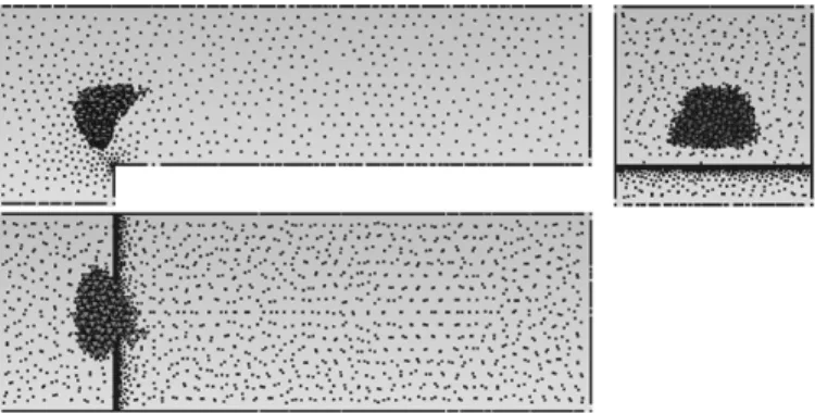
Fig. 2. Deepest set of tunnel202, xyz projections are shown. Points are the vertices of covering surface, nodes of Deepest set represented by tetrahedrons.
C. DLS Bisection
The base concept of DLS bisection is the division of the mesh along the deepest set of nodes. GPS method creates level-structures from an extremal node and indexes nodes level by level. Bandwidth of the solution is proportional to the size of the largest level. In geometrical view, the ordering starts from an extremal surface and creates onionskins through the mesh, and the bandwidth is proportional to the largest cutting surface. In case of a structured grid of a rectangle, the bandwidth of GPS solution is proportional to the smaller side, which is often optimal. The elements of Deepest set take place on a line which is perpendicular to the smaller side, furthermore the line separates the rectangle into two equal sized parts.
DLS can be obtained by the Level Structure() routine, starting the BFS from the Cover set, the resulting level structure will be the DLS structure. The Deepest set is the union of the three deepest levels in DLS. The method uses the three deepest levels, because the deepest level may contains only one node, and the base idea of the bisection is to cut the deepest area of the mesh. Using pseudo diameter routine, the method gets two endpoints of Deepest set, which have maximal distance from each other in the whole mesh(Deepest set is not necessarily connected). DLS-Based bisecting method generates the separating surface in two steps. In the first stage a set of nodes are obtained which have the same distance from the two endpoints of theDeepestset’s pseudo-diameter.
The resulting set is used during the second stage.The final set separates the mesh into two parts.
Fig. 3. sep2 of tunnel202, xyz projections are shown. Points are the vertices of covering surface, nodes of the separator represented by tetrahedrons.
// Get Separator
1 Level Structure(Cover, DLS) 2 P seudo Diameter(Deepest,(u, v)) 3 Level Structure({u}, LU)
4 Level Structure({v}, LV)
5 sep1 ={x:Level(x, LU)−Level(x, LV)∈ {0,1}}
6 P seudo Diameter(sep1,(u, v)) 7 Level Structure({u}, LU) 8 Level Structure({v}, LV)
9 sep2 ={x:Level(x, LU)−Level(x, LV)∈ {0,1}}
The resulting separator is parallel to the pseudo diameter of theDeepestset, but the separator not necessarily intersects the Deepest set. The correction step is responsible for placing the separator to the middle of theDeepestset. Separatorsep2is the set of nodes which have the same distance from the endpoints of the pseudo diameter ofsep1. If the Deepestset is closer to one of the two endpoints, the separator must be moved towards that point. All levels of the level-structure started from sep2, is equal to two separators which appear at the sides of sep2.
The correction phase removes the further node set from each level. The level is chosen as corrected separator which has largest intersection with Deepest set.
// Correction on Separator
1 dist u=M IN{Level(x, LU)|x∈Deepest}
2 dist v=M IN{Level(x, LV)|x∈Deepest}
3 if dist u < dist v
4 Level Structure({u}, LS1) 5 Level Structure({v}, LS2) 6 else
7 Level Structure({v}, LS1) 8 Level Structure({u}, LS2) 9 Level Structure(sep2, LSep) 10 for∀x∈LSep
11 ifLevel(x, LS1)> Level(x, LS2) 12 delete x f rom LSep
13 Separator = level L of LSep f or which
|L∩Deepest|is maximal
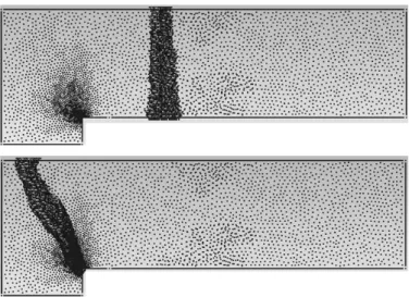
Fig. 4. Separator of tunnel100 before correction (up), and after (down).
The partition method is not completed by determining the separator surface, because our separator is a set of nodes, therefore the partition is ambiguous. Two parts are obtained by using theGrowsubroutine, but the separator and its nearest neighborhood still remains unpartitioned. Unpartitioned nodes are added to the smaller part. The method can be finished at this point, but the size balance is not guaranteed. A simple solution is to grow the smaller part till balance reached.
// Get parts from separator 1 s /∈Separator
2 Grow(s, Separator, part1) 3 s /∈Separator∪part1 4 Grow(s, Separator, part2) 5 rest={x:x /∈part1∪part2}
6 Add rest to the smaller part
7 Grow smaller part till balance reached III. RESULTS
Our test environment is based on GMSH[3], which is a three-dimensional finite element mesh generator with built- in pre- and post-processing facilities. In GMSH simple 3D models can be defined, meshed and partitioned. The covering surfaces are given as physical surfaces, which makes possible for our algorithm to get the cover of the mesh.
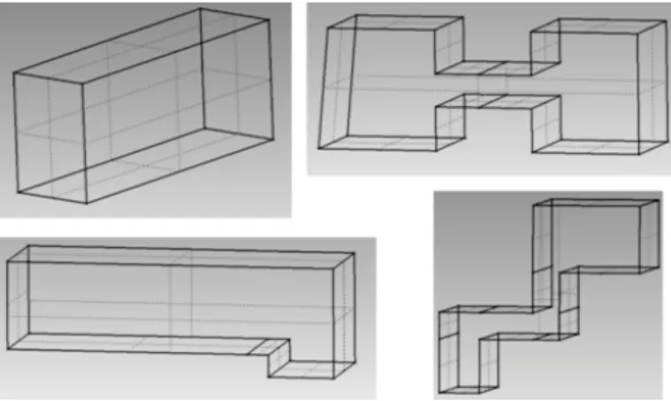
The test models are shown in Figure 5. Meshes generated from sgrid are structured grids of hexahedrons, from snake and weight unstructured tetrahedron-based meshes are generated with uniform density, in case of tunnel the density of the mesh is increased around the step.
A. Results
A comparison is shown in Table I between the DLS-Based and the METIS-recursive partitioning. The objective of the two partitioner is different, but there is no other known method, which minimizes the graph bandwidth of the resulting partitions, and METIS is one of the most popular solver.
Fig. 5. Test shapes. sgrid, weight (up), tunnel, snake(down)
For the structured brick-shaped problems, the DLS method provides average 28% better BW partition, with acceptable communication ratio (external reads / inner). The COMM ratio is better for larger problems, in case of sgrid4, which has 1M vertices, the COMM ratio is only 1,6%. The values depend on the ratio between the side lengths, but the tendencies are independent.
TABLE I
RESULTS OFDLS BASEDPARTITION
Problem N Orig BW MET BW MET COMM DLS BW DLS COMM
sgrid1 2200 221 181 0,0388 141 0,1216
sgrid2 16800 841 641 0,0192 479 0,0628
sgrid3 131200 3281 2517 0,0087 1719 0,0323
sgrid4 1036800 12961 9967 0,0045 6599 0,0164
snake100 7821 777 689 0,0254 531 0,079
snake038 158544 5701 5371 0,0074 4941 0,0095
tunnel202 18210 2353 1385 0,0292 1303 0,0262
tunnel100 191592 12525 5675 0,017 5949 0,027
weight045 4899 641 581 0,0169 311 0,1764
weight022 35922 2363 2131 0,0078 1411 0,0559
weight012 230891 8087 8785 0,0037 8785 0,0075
N: number of vertices. Orig BW: GPS BW for the whole mesh.
MET/DLS BW: BW of partitions.
MET/DLS COMM: number of outgoing edges / number of internal edges
The communication ratio (edge-cut ratio) is getting better when the mesh density is increased for all problem instances.
This is obvious because the cutting surface has N-1 dimension in case of an N dimensional mesh. This feature is important, because DLS computes a kind of N-1 dimensional surface, which separates the mesh into two parts. DLS-Based solutions can have unacceptable communication need for small meshes, for example weight045, where the COMM ratio is 17,5%.
Using DLS-Based bisection the resulting partitions have 40%
reduced graph bandwidth compared to the whole mesh, and create 20% better solutions than METIS. METIS minimizes the edge-cut and provides size-balance, the DLS-Based solutions have same size balance quality, however the edge-cut is several times higher. There is a tradeoff between graph bandwidth and communication need, and DLS creates partitions with higher COMM ratio to provide reduced graph bandwidth.
DLS reduces the bandwidth by 40-50% by separating the mesh along the Deepest set, in case of tunnel geometry the METIS solution has the same reduction ratio, for tunnel202 the partition is nearly similar and DLS has better COMM ratio, for tunnel100 the METIS solution has better graph bandwidth.
The difference between the traditional methods and DLS- Based partitioning can be observed on Figure 6, where the separator of weight022 is shown. DLS-Based bisection cuts the weight shape in longitudinal direction, instead of choosing the small edgecut between the two weights. This partition leads to 34% better graph bandwidth reduction with 5,6%
COMM ratio.
Fig. 6. Separator of weight022.
If the DLS separator do not provide size balance, the proposed method grows the smaller part until the balance is reached. This strategy can increases the graph bandwidth of the solution. For weight012 the BW of the resulting parts are 6741 without size balance, and 8785 after, because the balance leads to a quasi similar partition to METIS. The graph bandwidth of the parts can be higher than the original mesh, because GPS is a heuristic algorithm, and the graph bandwidth mainly depends on the largest cutting surface.
B. Bounded BW partitioning
The proposed method is created for providing partitions which meet constraints on the graph bandwidth. If the original mesh has larger GPS bandwidth than the given bound, the method bisects the mesh. Parts can be bisected if the constraint on the bound is still unsatisfied. The constraints on graph bandwidth can be reached in less bisection steps with DLS- Based method, than with other traditional partitioners.
IV. CONCLUSIONS
In this paper a novel partitioning problem is presented, which is a combination of the classical partitioning problem, and the bandwidth reduced node ordering on the resulting parts. The motivation of this partitioning problem is based on FPGA designs, where the graph bandwidth of the input parts has to be below a bound. The proposed solver uses the covering node set of the given mesh, which contains
information from the geometry without space coordinates. The covering surface is often given (physical simulations), but is not used by traditional partitioners. The proposed method is an example of using covering surface in partitioning techniques.
The components of the DLS-Based method are operations on node sets, which operations use spatial waves to compute abstract surfaces (node sets) inside the mesh.
The results show that the proposed partitioning algorithm creates partitions with better graph-bandwidth quality than METIS, with acceptable edgecut. The size-balancing steps of the method should be improved, because the graph-bandwidth quality of the solution can be damaged.
V. ACKNOWLEDGEMENT
This research project supported by the J´anos Bolyai Re- search Scholarship of the Hungarian Academy of Sciences and OTKA Grant No. K84267. The support of the grants TMOP- 4.2.1.B-11/2/KMR-2011-0002 and TMOP-4.2.2/B-10/1-2010- 0014 is also acknowledged.
REFERENCES
[1] N.E. Gibbs, W.G. Poole, P.K. Stockmeyer, An algorithm for reducing the bandwidth and profile of sparse matrix, SIAM Journal on Numerical Analysis 13 (2) 236-250 (1976)
[2] G. Karypis and V. Kumar. A fast and highly quality multilevel scheme for partitioning irregular graphs. SIAM Journal on Scientific Computing Vol. 20, No. 1, pp. 359-392 (1998)
[3] C. Geuzaine and J.-F. Remacle. Gmsh: a three-dimensional finite element mesh generator with built-in pre- and post-processing facilities. Interna- tional Journal for Numerical Methods in Engineering, Volume 79, Issue 11, pages 1309-1331, (2009)
[4] www.alpha-data.com