arXiv:1804.05815v1 [astro-ph.HE] 16 Apr 2018

(1)

arXiv:1804.05815v1 [astro-ph.HE] 16 Apr 2018

ABSOLUTE DISTANCES TO NEARBY TYPE IA SUPERNOVAE VIA LIGHT CURVE FITTING METHODS

J. VINKO´,^{1, 2, 3}A. ORDASI,¹T. SZALAI,²K. S ÁRNECZKY,¹E. B ÁNYAI,¹I. B. BÍRO´,⁴ T. BORKOVITS,^{4, 1, 5}T. HEGEDUS¨ ,⁴ G. HODOSAN´ ,^{1, 5, 6}J. KELEMEN,¹P. KLAGYIVIK,^{5, 1, 7, 8}L. KRISKOVICS,¹E. KUN,⁹G. H. MARION,³G. MARSCHALKO´,⁵L. MOLNAR´ ,¹

A. P. NAGY,²A. P ´AL,¹J. M. SILVERMAN,^{3, 10}R. SZAKATS´ ,¹E. SZEGEDI-ELEK,¹ P. SZEKELY´ ,⁹ A. SZING,⁴K. VIDA,¹AND

J. C. WHEELER³

1Konkoly Observatory of the Hungarian Academy of Sciences, Konkoly-Thege ut 15-17, Budapest, 1121, Hungary

2Department of Optics and Quantum Electronics, University of Szeged, Dom ter 9, Szeged, 6720, Hungary

3Department of Astronomy, University of Texas at Austin, 2515 Speedway, Austin, TX, USA

4Baja Observatory of the University of Szeged, Szegedi ut KT 766, Baja, 6500, Hungary

5Department of Astronomy, Eötvös Loránd University, Pazmany setany 1/A, Budapest, Hungary

6Centre for Exoplanet Science, School of Physics and Astronomy University of St Andrews, St Andrews KY16 9SS, UK

7Instituto de Astrofsica de Canarias, C. Va Lctea S/N, 38205 La Laguna, Tenerife, Spain

8Universidad de La Laguna, Dept. de Astrofsica, 38206 La Laguna, Tenerife, Spain

9Department of Experimental Physics, University of Szeged, Dom ter 9, Szeged, 6720, Hungary

10Samba TV, 123 Townsend St., San Francisco, CA, USA

(Received; Revised; Accepted) Submitted to PASP

ABSTRACT

We present a comparative study of absolute distances to a sample of very nearby, bright Type Ia supernovae (SNe) derived from high cadence, high signal-to-noise, multi-band photometric data. Our sample consists of four SNe: 2012cg, 2012ht, 2013dy and 2014J. We present new homogeneous, high-cadence photometric data in Johnson-CousinsBV RI and Sloang^′r^′i^′z^′bands taken from two sites (Piszkesteto and Baja, Hungary), and the light curves are analyzed with publicly available light curve fitters (MLCS2k2, SNooPy2 and SALT2.4). When comparing the best-fit parameters provided by the different codes, it is found that the distance moduli of moderately-reddened SNe Ia agree within.0.2mag, and the agreement is even better (.0.1mag) for the highest signal-to-noiseBV RIdata. For the highly-reddened SN 2014J the dispersion of the inferred distance moduli is slightly higher. These SN-based distances are in good agreement with the Cepheid distances to their host galaxies. We conclude that the current state-of-the-art light curve fitters for Type Ia SNe can provide consistent absolute distance moduli having less than∼0.1 – 0.2 mag uncertainty for nearby SNe. Still, there is room for future improvements to reach the desired∼0.05mag accuracy in the absolute distance modulus.

Keywords:(stars:) supernovae: individual (SN 2012cg, SN 2012ht, SN 2013dy, SN 2014J) — galaxies: distances and redshifts

Corresponding author: J. Vink´o vinko@konkoly.hu

(2)

1. INTRODUCTION

Getting reliableabsolutedistances is of immense importance in observational astrophysics. Supernovae (SNe) in particular play a central role in establishing the extragalactic distance ladder. Distances to Type Ia SNe are essential data for studying the expansion of the Universe (Riess et al. 1998;

Perlmutter et al. 1999; Astier et al. 2006; Riess et al. 2007;

Wood-Vasey et al. 2007;Kessler et al. 2009;Guy et al. 2010;

Conley et al. 2011; Betoule et al. 2014; Rest et al. 2014;

Scolnic et al. 2014). SNe Ia are also especially important objects for measuring the Hubble-parameterH0(Riess et al.

2011,2016;Dhawan et al. 2017), and they play a key role in testing current cosmological models (Benitez-Herrera et al.

2013;Betoule et al. 2014). Their importance has even been strengthened since the release of the cosmological parameters from the Planck mission (Planck Collaboration et al.

2014,2015), which turned out to be slightly in tension with the current implementation of the SN Ia distance measurements (seeRiess et al. 2016, and references therein).

It must be emphasized that the majority of cosmological studies userelativedistances to moderate- and high-redshift SNe Ia to derive the cosmological parameters (Ωm,ΩΛ,w, etc). From this point of view there is no need for having absolute distances, because the relative distances between different SNe/galaxies can be obtained with much better accuracy, especially if the galaxy is in the Hubble-flow (z&0.1).

On the other hand, having accurate absolute distances to the nearby galaxies that are not part of the Hubble-flow is very important an astrophysical point of view. Getting reliable estimates for the physical parameters of such galaxies and the objects within them is possible only if we have reliable absolute distances on extragalactic scales.

Thus, investigating the nearest SNe Ia (withinz . 0.01) can provide valuable information for various reasons. For example, distances to their host galaxies can be relatively easily determined by several methods, thus, the SN-based distances can be compared directly to those derived independently by using other types of objects and/or methods.

Such very nearby galaxies might also serve as “anchors” in the cosmic distance ladder (e.g. NGC 4258, seeRiess et al.

2011,2016), which play an essential role in measuringH0. The popularity of SNe Ia as extragalactic distance estima- tors is mostly due to the fact that their absolute distances can be derived via fitting light curves (LCs) of “normal” Ia events. The LCs of such events obey the empirical Phillips- relation, i.e. intrinsically brighter SNe have more slowly de- clining LCs in the optical bands (Pskovskii 1977; Phillips 1993). Even though nowadays SNe Ia seem to be even better standard candles in the near-infrared (NIR) regime than in the optical (Friedman et al. 2015;Shariff et al. 2016;

Weyant et al. 2017), obtaining rest-frame NIR LCs for SNe Ia, except for the nearest and brightest ones, can be chal-

lenging. Thus, photometric data taken in rest-frame optical bands can still provide valuable information regarding distance measurements on the extragalactic scale.

One of the main motivations of the present paper is to get absolute distances to some of the nearest and brightest recent SNe Ia by fitting homogeneous, high-cadence, high S/N photometric data with public, widely-used LC-fitting codes. We selected four nearby Type Ia SNe for this project: 2012cg, 2012ht, 2013dy and 2014J. All of them occured in the local Universe, and they were discovered relatively early (more than 1 week before B-band maximum). We have obtained new, densely sampled photometric measurements for each of them in various optical bands, which resulted in light curves extending from pre-maximum epochs up to the end of the photospheric phase. These objects, along with SN 2011fe, belong to the 10 brightest SNe Ia in last decade that were accessible from the northern hemisphere. However, unlike SN 2011fe, all of them were significantly reddened by dust either in the Milky Way or in their hosts, which enabled us to test the performance of the LC-fitters in case of reddened SNe. In addition, their very low redshift (z < 0.01) eliminated the necessity for K-correction, which could be another possible cause for systematic errors when comparing photometry of SNe having significantly different redshifts (Saunders et al. 2015). It is also important to note that three out of four SNe in our sample have Cepheid-based distances obtained byHST/WFC3, and they were recently used in calibratingH0with an unprecedented 2.4 percent accuracy (Riess et al. 2016).

The basic parameters for the program SNe are collected in Table1.

In the following we briefly describe the observations (Sec- tion2) and the LC-fitting codes applied (Section3). Section4 presents the results from the LC fitting, which are discussed further in Section5. Section6summarizes the main results and conclusions.

2. OBSERVATIONS

Photometry of the target SNe have been carried out at two sites, located∼ 200km apart: at the Piszk´estet˝o station of Konkoly Observatory, Hungary, and at Baja Observatory of the University of Szeged, Hungary. At Konkoly the data were taken with the 0.6m Schmidt telescope through Bessell BV RIfilters. At Baja the observations were carried out with the 0.5m BART telescope equipped with Sloang^′r^′i^′z^′ filters. SeeVink´o et al. (2012) for more details on these two instruments.

All data have been reduced using standard IRAF¹ rou- tines. Transformation to the standard photometric systems

1IRAF is distributed by the National Optical Astronomy Observatories, which are operated by the Association of Universities for Research in As-

(3)

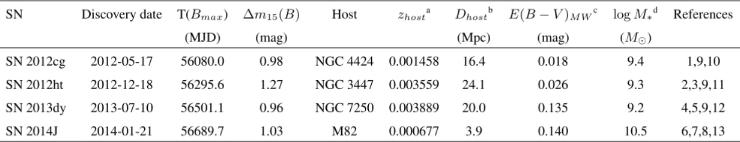
Table 1.Basic data for the studied SNe

SN Discovery date T(Bmax) ∆m15(B) Host zhosta Dhostb E(B−V)M Wc logM∗d

References

(MJD) (mag) (Mpc) (mag) (M⊙)

SN 2012cg 2012-05-17 56080.0 0.98 NGC 4424 0.001458 16.4 0.018 9.4 1,9,10

SN 2012ht 2012-12-18 56295.6 1.27 NGC 3447 0.003559 24.1 0.026 9.3 2,3,9,11

SN 2013dy 2013-07-10 56501.1 0.96 NGC 7250 0.003889 20.0 0.135 9.2 4,5,9,12

SN 2014J 2014-01-21 56689.7 1.03 M82 0.000677 3.9 0.140 10.5 6,7,8,13

aHost galaxy redshift, adopted from NED

bCepheid distances fromRiess et al.(2016); mean redshift-independent distance from NED for SN 2014J cMilky Way reddening based on IRAS/DIRBE maps (Schlafly & Finkbeiner 2011)

dHost galaxy stellar mass based on SED fitting with Z-PEG (Le Borgne & Rocca-Volmerange 2002)

NOTE— References: (1):Silverman et al.(2012); (2):Yusa et al.(2012); (3):Yamanaka et al.(2014); (4):Zheng et al. (2013); (5):Pan et al.

(2015); (6):Fossey et al. (2014); (7):Zheng et al. (2014); (8):Marion et al. (2015a) ; (9):Riess et al. (2016); (10):Cort´es et al. (2006) ; (11):Mazzei et al.(2017); (12):Pan et al.(2015); (13):Dale et al.(2007)

(4)

(Johnson-Cousins/Vega and Sloan/AB for the BV RI and g^′r^′i^′z^′ data, respectively) was computed using catalogued Sloan-photometry for local tertiary standard stars. In the fields of SN 2012cg and SN 2012ht theBV RI magnitudes for the local standards were calculated from their catalogued g^′r^′i^′z^′magnitudes using the calibration given byJordi et al.

(2006). For SN 2013dy and 2014J the estimated BV RI magnitudes obtained this way were cross-checked by ob- serving Landolt standard fields on a photometric night and re-calibrating the local standards using the zero-points from the Landolt standards. Finally, allBV RI photometry were cross-compared to the Pan-STARRS (PS1) magnitudes² of the local standards stars, and small (.0.1mag) shifts were applied when needed to bring all the photometry to the same zero-point. The finalBV RImagnitudes for the local comparison stars are shown in the Appendix (Table11, 13,15 and18).

Photometry of the SNe was obtained via PSF-fitting using DAOPHOT. The resulting instrumental magnitudes were transformed to the standard systems by applying linear color terms, and the zero points of the transformation are tied to the magnitudes of the local comparison stars.

The final LCs were compared with other published, independent photometry for each SNe, except for SN 2012ht, where no other available photometry was found. We used the data given byMarion et al.(2015b),Pan et al.(2015) and Marion et al.(2015a) for SN 2012cg, 2013dy and 2014J, respectively. A∼0.1mag systematic difference was identified between theB-band LCs of the heavily-reddened SN 2014J, which was corrected by shifting our data to match those published byMarion et al.(2015a). No such systematic offsets between our data and those from others were found for the re- maining three SNe. The final photometric data can be found in the Appendix, in Tables12,14,16,17and19.

3. ANALYSIS

We applied three SN Ia LC-fitters for this study: MLCS2k2³ (Riess et al. 1998; Jha et al. 1999; Jha, Riess & Kirshner 2007), SALT2⁴version 2.4 (Guy et al. 2007,2010;Betoule et al.

2014) and SNooPy2⁵ (Burns et al. 2011;Burns et al. 2014).

All these, in principle, rely on the Phillips-relation but each code uses different parametrization for fitting the light curve shape and each has different sets of calibrating SNe (“training sets”). There are also other implementations, like SiFTO (Conley et al. 2008) or BayeSN (Mandel et al. 2011), but the

tronomy, Inc., under cooperative agreement with the National Science Foun- dation.

2http://archive.stsci.edu/panstarrs/search.php

3http://www.physics.rutgers.edu/˜saurabh/mlcs2k2/

4http://supernovae.in2p3.fr/salt/doku.php

5http://csp.obs.carnegiescience.edu/data/snpy/snpy

first three listed above have been used most frequently in the literature.

Conley et al.(2008) categorized such codes as either “pure LC-fitters” or “distance calculators”. Distance calculators can provide the true absolute distance as a fitting parameter, but they require a training set of SNe having independently obtained absolute distances. Since building such a training set is non-trivial, the calibration of such codes is usually based on a relatively small number of objects. On the contrary, LC-fitters can predict only relative distances, but they can be calibrated using a much larger sample of objects having much more accurate relative distances. Regarding the three codes applied in our study, MLCS2k2 and SNooPy2 are distance calculators, while SALT2 is an LC-fitter, even though it is possible to derive absolute distances from the SALT2 fitting parameters, if needed.

MLCS2k2 (Jha, Riess & Kirshner 2007) uses the following SN Ia LC model:

mx(ϕ) = M_x⁰+µ0+ηxA⁰_V +Px∆ +Qx∆², (1) whereϕ = t−Tmaxis the SN phase in days,Tmaxis the moment of maximum light in the B-band, mx is the observed magnitude in thex-band (x = B, V, R, I), M_x⁰(ϕ) is the fiducial SN Ia absolute LC in the same band, µ0

is the true (reddening-free) SN distance modulus, ηx = ζx(αx+βx/RV)gives the time-dependent interstellar reddening,RV andA⁰_V are the ratio of total-to-selective absorption andV-band extinction at maximum light, respectively,

∆is the main LC parameter, andPx(ϕ)andQx(ϕ)are tabu- lated functions of the SN phase (“LC-vectors”). The absolute magnitudes of SNe in MLCS2k2 have been calibrated using relative distances of more than 150 SNe in the Hubble-flow assumingH0= 65km s⁻¹Mpc⁻¹, but later they were tied to Cepheid distances of a smaller sample of SNe Ia host galaxies (Riess et al. 2005).

Contrary to MLCS2k2, SALT2 models the whole spectral energy distribution (SED) of a SN Ia as

Fλ(ϕ) = x0·[M0(ϕ, λ)+x1M1(ϕ, λ)] exp[C·CL(λ)], (2) whereFλ(ϕ)is the phase-dependent rest-frame flux density, M⁰(ϕ, λ),M¹(ϕ, λ)andCL(λ)are the SALT2 trained vectors. The free parametersx0,x1andCare the normalization- , stretch- and color parameters, respectively.

Being an LC-fitter, SALT2 does not contain the distance as a fitting parameter. Instead, the distance modulus can be calculated from the following equation (Conley et al. 2011;

Betoule et al. 2014;Scolnic & Kessler 2016):

µ0 = m^∗B−MB+αx1−βC. (3) For the nuisance parametersα, β andMB we adopted the calibration byBetoule et al.(2014):MB=−19.17±0.038,

(5)

α = 0.141±0.006,β = 3.099±0.075, and derived the distance moduli from the fitting parameters via Monte-Carlo simulations.

One of the great advantages of SALT2 is that it can be relatively easily applied to data taken in practically any photometric system provided the filter transmission functions are loaded into the code. Because of this and many other reasons, SALT2 became very popular recently, and it was used in most papers dealing with SN Ia light curves (e.g.

Betoule et al. 2014;Mosher et al. 2014; Scolnic et al. 2014;

Rest et al. 2014; Saunders et al. 2015; Walker et al. 2015;

Riess et al. 2016;Zhang et al. 2017). We utilized the built- in “Landolt-Bessell” and “SDSS” filter sets for fitting our BV RIandg^′r^′i^′z^′data, respectively.

While applying SNooPy2, we adopted the default “EBV- model” as a proxy for a SN Ia LC:

mX(ϕ) = TY +MY +µ0+KXY +

RXE(B−V)M W +RYE(B−V)host, (4) whereX, Y denote the filter of the observed data and the template light curve, respectively, mX(ϕ) is the observed LC in filterX,TY(ϕ,∆m15)is the template LC as a function of time,∆m15is the generalized decline-rate parameter associated with the∆m15(B)parameter byPhillips(1993), MY(∆m15)is the absolute magnitude of the SN in filterY as a function of∆m15,µ0is the reddening-free distance modulus in magnitudes, E(B −V) is the color excess due to interstellar extinction either in the Milky Way (“MW”), or in the host galaxy, RX,Y are the reddening slopes in filter X orY andKXY(t, z)is the cross-band K-correction that matches the observed broad-band magnitudes of a redshifted (z&0.01) SN taken with filterXto a template SN LC in fil- terY. Since all our SNe had very low redshift (z <0.01) we always setX = Y and neglected the K-corrections, which greatly simplified the analysis of those objects.

SNooPy2 offers two sets of templates which cover different filter bands. We utilized the Prieto-templates (Prieto et al.

2006) for fitting theBV RILCs, while for theg^′r^′i^′z^′data we selected the built-in CSP-templates which include theg- , r- and i-bands. For SN 2012cg, 2012ht and 2013dy we adopted the standardRV = 3.1reddening slope (corresponding to thecalibration=2mode in SNooPy2), while for SN 2014J, which suffered from strong non-standard reddening, we tested both theRV ∼1.0(calibration=6) and RV ∼1.5(calibration=3) settings. These different calibrations are detailed inFolatelli et al.(2010).

All of these codes fit the template LCs to the observed ones viaχ²-minimization, taking into account photometric errors as inverse weights. The optimized parameters are as follows:

• Tmax: the moment of maximum light in theB-band (MJD)

8 9 10 11 12 13 14 15 16

-20 -10 0 10 20 30 40 50

Magnitude

Days from B-maximum SN 2012cg BVRI fit with MLCS2k2

B V R I

8 9 10 11 12 13 14 15 16

-20 -10 0 10 20 30 40 50

Magnitude

Days from B-maximum SN 2012cg BVRI fit with SNooPy2

B V R I

8 9 10 11 12 13 14 15 16

-20 -10 0 10 20 30 40 50

Magnitude

Days from B-maximum SN 2012cg BVRI fit with SALT2.4

B V R I

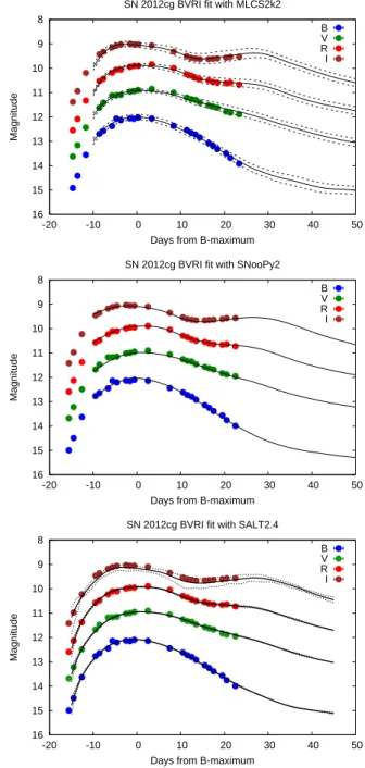
Figure 1. The fitting of SN 2012cg light curves, after correcting for Milky Way extinction. Top: MLCS2k2 templates; middle: SNooPy2 templates; bottom: SALT2.4 templates. Dashed and dotted lines represent the template uncertainties for MLCS2k2 and SALT2.4, respectively.

• A^host_V : the interstellar extinction in the host galaxy in V-band (magnitude)

• µ⁰: extinction-free distance modulus (magnitude)

• ∆: light curve shape parameter (MLCS2k2)

• ∆m15: light curve shape parameter (SNooPy2)

• mB: peak brightness inB-band (SALT2, magnitude)

(6)

• x⁰: light curve normalization parameter (SALT2)

• x1: light curve shape parameter (SALT2)

• C: color parameter (SALT2)

Uncertainties of the fitting parameters were calculated via the standard analysis of the Hessian matrix of the χ²- hypersurface.

A particularly important goal of this study was checking the consistency of the distance moduli obtained from different photometric systems, i.e. to cross-compare the results from Johnson-CousinsBV RI and Sloan g^′r^′i^′z^′. SALT2 and SNooPy2 are capable of handling LCs taken in g^′r^′i^′ bands, but not in thez^′-band. The publicly released version of MLCS2k2 contains only templates inU BV RI-bands. In order to make the analysis as complete as possible, we mi- grated the MLCS2k2U BV RItemplates to cover theg^′r^′i^′z^′ filters. Details on this step are given in the Appendix.

Several studies (e.g.Hicken et al. 2009;Kelly et al. 2010;

Lampeitl et al. 2010; Sullivan et al. 2010) pointed out the correlation between SN Ia peak brightnesses and host galaxy stellar masses: SNe in more massive (Mstellar &10¹⁰M⊙) galaxies tend to be slightly brighter at peak compared to SNe in less massive hosts. We discuss the implication of this correlation on the derived distances in Section4.

Previously the comparison of MLCS2k2 and SALT2 was presented by Kessler et al. (2009), who analyzed the first- season data from the SDSS-II SN survey. They found moderate disagreement (at the∼ 0.1 – 0.2 mag level) between the distance moduli for their nearby SN sample calculated by the two codes. A similar result was obtained by Vink´o et al.(2012) when fitting theBV RI data for the extremely well-observed SN 2011fe: the distance moduli given by MLCS2k2 and SALT2 differ by∼0.16mag. In the rest of the paper we make a similar comparison for our SN sample by involving SNooPy2 and using data taken in different photometric systems.

We would like to emphasize that it is not intended to judge which code is superior over the others. We use these codes

“as is” without any attempts to fine-tune or retrain their calibrations to get better match with any particular data, except for bringing them onto the same distance scale (see below).

4. RESULTS

This section summarizes the fits obtained from the different methods, and compare the results with those from previous studies, where applicable. Note that the different methods use different Hubble-parameters (H0) for their relative distance scales: MLCS2k2, SNooPy2 and SALT2.4 assume H0 = 65, 72 and 68 km s⁻¹ Mpc⁻¹, respectively. In order to bring the reported distance moduli onto the same scale, all of them have been corrected toH0 = 73km s⁻¹Mpc⁻¹

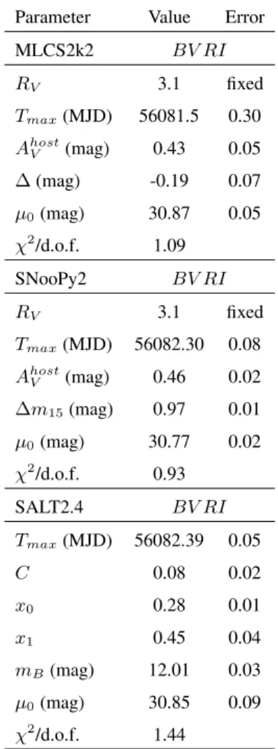
Table 2.Best-fit parameters for SN 2012cg Parameter Value Error

MLCS2k2 BV RI

RV 3.1 fixed

T^max(MJD) 56081.5 0.30 A^hostV (mag) 0.43 0.05

∆(mag) -0.19 0.07

µ0(mag) 30.87 0.05

χ²/d.o.f. 1.09

SNooPy2 BV RI

R^V 3.1 fixed

Tmax(MJD) 56082.30 0.08 A^hostV (mag) 0.46 0.02

∆m15(mag) 0.97 0.01

µ0(mag) 30.77 0.02

χ²/d.o.f. 0.93

SALT2.4 BV RI

Tmax(MJD) 56082.39 0.05

C 0.08 0.02

x0 0.28 0.01

x1 0.45 0.04

mB(mag) 12.01 0.03

µ0(mag) 30.85 0.09

χ²/d.o.f. 1.44

(Riess et al. 2016). The tables below contain these homog- enized distance moduli. The cross-comparison of the distances obtained by these codes is further discussed in Sec- tion5.

4.1. SN 2012cg

Previous photometry of SN 2012cg has been presented and analyzed by Silverman et al. (2012), Munari et al. (2013), Amanullah et al.(2015) andMarion et al.(2015b). Table2 lists the optimum parameters found by the different LC fitters applied by us. Comparing their values with the ones given by the previous studies, it is seen that they are generally consistent. There is only a slight tension between the estimated values of the extinction within the host: the results in Table2 implyE(B−V)host=A^host_V /RV = 0.14±0.02mag, while Silverman et al. (2012) and Marion et al. (2015b) obtained E(B−V)host∼0.18±0.05mag which is marginally consistent with our results. Our lower reddening/extinction is closer toE(B−V)host∼0.13mag estimated byAmanullah et al.

(2015). For the distance modulus, the parameter that we

(7)

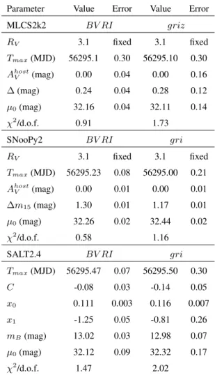
Table 3.Best-fit parameters for SN 2012ht

Parameter Value Error Value Error

MLCS2k2 BV RI griz

RV 3.1 fixed 3.1 fixed

T^max(MJD) 56295.1 0.30 56295.10 0.30 A^hostV (mag) 0.00 0.04 0.00 0.16

∆(mag) 0.24 0.04 0.28 0.12

µ0(mag) 32.16 0.04 32.11 0.14

χ²/d.o.f. 0.91 1.73

SNooPy2 BV RI gri

R^V 3.1 fixed 3.1 fixed

Tmax(MJD) 56295.23 0.08 56295.00 0.21 A^hostV (mag) 0.00 0.01 0.00 0.01

∆m15(mag) 1.30 0.01 1.17 0.01

µ0(mag) 32.26 0.02 32.44 0.02

χ²/d.o.f. 0.58 1.16

SALT2.4 BV RI gri

Tmax(MJD) 56295.47 0.07 56295.50 0.30

C -0.08 0.03 -0.14 0.05

x0 0.111 0.003 0.116 0.007

x1 -1.25 0.05 -0.81 0.26

mB(mag) 13.02 0.03 12.98 0.07

µ0(mag) 32.12 0.09 32.32 0.17

χ²/d.o.f. 1.47 2.02

focus on in this work, Munari et al.(2013) obtainedµ0 = 30.95assumingE(B−V) = 0.18mag, which, after correcting toE(B−V) = 0.14mag, corresponds toµ0= 30.83in very good agreement with our results presented in Table2.

The light curves of SN 2012cg are plotted together with the models from the different LC fitters in Fig.1.

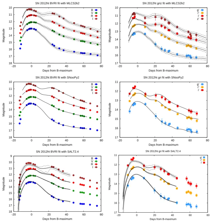
4.2. SN 2012ht

A photometric study of SN 2012ht has been presented byYamanaka et al. (2014). From their BV RI photometry they have estimated the following parameters: Tmax(B) = 56295.6±0.6,∆m15(B) = 1.39mag andE(B−V)host∼0 mag. As seen from Table3, these are in good agreement with our results. The light curves together with the best-fit models can be found in Fig.2. It is seen that theBV RI data that have lower measurement errors could be fit better: their re- ducedχ²values (Table3) are lower than those of theg^′r^′i^′z^′ data.

In order to test the consistency of the photometric calibration of our BV RI and g^′r^′i^′ data, simultaneous fits to

Table 4.Best-fit parameters for SN 2013dy

MLCS2k2 BV RI griz

∆(mag) -0.23 0.06 -0.30 0.12

µ0(mag) 31.51 0.06 31.65 0.13

χ²/d.o.f. 1.34 1.91

SNooPy2 BV RI gri

∆m15(mag) 0.96 0.01 0.80 0.01

µ0(mag) 31.52 0.03 31.44 0.04

χ²/d.o.f. 0.99 3.45

SALT2.4 BV RI gri

Tmax(MJD) 56501.44 0.06 56501.99 0.14

C 0.089 0.025 0.03 0.03

x0 0.154 0.004 0.169 0.006

x1 0.695 0.044 1.51 0.12

mB(mag) 12.67 0.03 12.57 0.04

µ0(mag) 31.52 0.09 31.72 0.11

χ²/d.o.f. 0.76 2.70

the combined LCs were also computed with SNooPy2 and SALT2.4 (MLCS2k2 was trained only onBV RI data, so that code was not applied in this test). As expected, these fits produced slightly higherχ²values than the fits to theBV RI LCs alone, but their best-fit parameters were consistent with the ones listed in Table3. In particular, the distance modulus from the combined fits turned out to beµ0 = 32.20±0.01 mag (χ²/d.o.f=0.83) from SNooPy2, while from SALT2.4 it is32.13±0.08mag (χ²/d.o.f.=2.81). These parameters are closer to those obtained from fitting theBV RILCs than those from fitting theg^′r^′i^′z^′ data, probably because of the lower measurement uncertainties of the former.

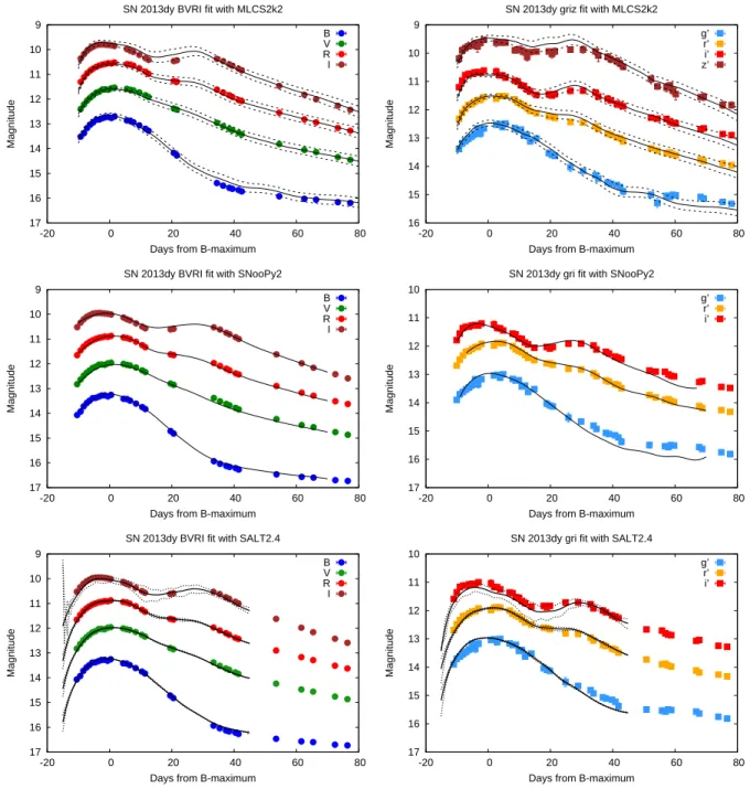
4.3. SN 2013dy

Light curves of SN 2013dy have been published recently by Pan et al. (2015) (P15) and Zhai et al. (2016) (Z16) in the BV RIriZY JH and U BV RI bands, respectively.

Zhai et al. (2016) also presented photometry obtained by Swift/UVOT.

(8)

10 11 12 13 14 15 16 17 18

-20 0 20 40 60 80

Magnitude

Days from B-maximum SN 2012ht BVRI fit with MLCS2k2

B V R I

10 11 12 13 14 15 16 17

-20 0 20 40 60 80

Magnitude

Days from B-maximum SN 2012ht griz fit with MLCS2k2

g’

r’

i’

z’

10 11 12 13 14 15 16 17 18

-20 0 20 40 60 80

Magnitude

Days from B-maximum SN 2012ht BVRI fit with SNooPy2

B V R I

11 12 13 14 15 16 17

-20 0 20 40 60 80

Magnitude

Days from B-maximum SN 2012ht gri fit with SNooPy2

g’

r’

i’

9 10 11 12 13 14 15 16 17 18

-20 0 20 40 60 80

Magnitude

Days from B-maximum SN 2012ht BVRI fit with SALT2.4

B V R I

11

12

13

14

15

16

17

-20 0 20 40 60 80

Magnitude

Days from B-maximum SN 2012ht gri fit with SALT2.4

g’

r’

i’

Figure 2.The fitting of the light curves of SN 2012ht, after correcting for Milky Way extinction. Top row: MLCS2k2; middle row: SNooPy2;

bottom row: SALT2.4; left column:BV RIdata; right column:g^′r^′i^′z^′data.

Pan et al. (2015) applied the SNooPy2 code to fit their full BV RIriZY JH dataset simultaneously, and obtained Tmax(B) = 56501.1, ∆m15 = 0.886±0.006, E(B − V)host = 0.206±0.005mag andµ0 = 31.49±0.01mag.

Comparing these values with those in Table4it is apparent that the results ofPan et al.(2015) are close to the ones obtained in the present study, although the differences somewhat exceed the formal errors given by SNooPy2. Compar- ing the best-fit values of the common parameters obtained from different methods, e.g. A^host_V orµ0, it is seen that they also deviate much more than the uncertainties given by the

codes. Thus, it is suspected that the formal parameter errors, especially those reported by SNooPy2, are underestimated, and the true uncertainties should be higher. Keeping this in mind, the solutions presented in Table4are entirely consistent with the LC fit given byPan et al.(2015). The fit of the model LCs to the data can be seen in Fig.3.

We re-analyzed theBV RIlight curves of SN 2013dy from bothPan et al. (2015) and Zhai et al. (2016) with all three methods applied in this paper in order to cross-compare the results from fitting measurements taken independently on the same SN. We assumedRV = 3.1for all fits, as earlier. The

(9)

9 10 11 12 13 14 15 16 17

-20 0 20 40 60 80

Magnitude

Days from B-maximum SN 2013dy BVRI fit with MLCS2k2

B V R I

9 10 11 12 13 14 15 16

-20 0 20 40 60 80

Magnitude

Days from B-maximum SN 2013dy griz fit with MLCS2k2

g’

r’

i’

z’

9 10 11 12 13 14 15 16 17

-20 0 20 40 60 80

Magnitude

Days from B-maximum SN 2013dy BVRI fit with SNooPy2

B V R I

10 11 12 13 14 15 16 17

-20 0 20 40 60 80

Magnitude

Days from B-maximum SN 2013dy gri fit with SNooPy2

g’

r’

i’

9 10 11 12 13 14 15 16 17

-20 0 20 40 60 80

Magnitude

Days from B-maximum SN 2013dy BVRI fit with SALT2.4

B V R I

10 11 12 13 14 15 16 17

-20 0 20 40 60 80

Magnitude

Days from B-maximum SN 2013dy gri fit with SALT2.4

g’

r’

i’

Figure 3.The same as Fig.2but for SN 2013dy.

results are shown in Table5. It is seen that the consistency between the distance moduli from the three methods is excellent for all data. Overall, the distance moduli from the Konkoly data differ by less than∼ 1σ (. 0.1 mag) from both the P15 and Z16 results. Also, it is seen from Table5 that similar amount of dispersion in the distance moduli derived by the different codes from the same dataset appears for the P15 and Z16 LCs as well as for our data, which suggests that this dispersion is probably not simply due to photometric calibration issues, at least for theBV RIdata.

In addition, we also modeled the combinedBV RI+g^′r^′i LCs as in the case for SN 2012ht. The resulting distance

moduli areµ0 = 31.45±0.01mag (χ²/d.o.f.=2.92) from SNooPy2 andµ0= 31.54±0.07mag (χ²/d.o.f.=2.11) from SALT2.4. Again, these results are in good agreement with those listed in Table4, even though theχ²values of the combined fits are somewhat higher but still acceptable (note again that the uncertainty ofµ0reported by SNooPy2 is underestimated).

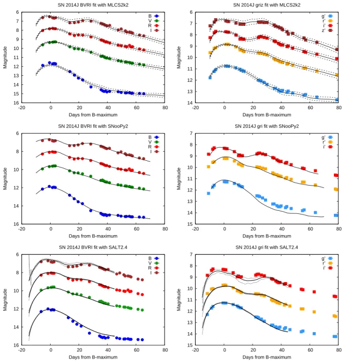
4.4. SN 2014J

As seen in Table 6, the LCs of SN 2014J have been fit with two different models assuming different reddening laws for the host galaxy in MLCS2k2 and SNooPy2. This was

(10)

6 7 8 9 10 11 12 13 14 15 16

-20 0 20 40 60 80

Magnitude

Days from B-maximum SN 2014J BVRI fit with MLCS2k2

B V R I

6 7 8 9 10 11 12 13 14

-20 0 20 40 60 80

Magnitude

Days from B-maximum SN 2014J griz fit with MLCS2k2

g’

r’

i’

z’

6

8

10

12

14

16

-20 0 20 40 60 80

Magnitude

Days from B-maximum SN 2014J BVRI fit with SNooPy2

B V R I

7 8 9 10 11 12 13 14 15

-20 0 20 40 60 80

Magnitude

Days from B-maximum SN 2014J gri fit with SNooPy2

g’

r’

i’

6

8

10

12

14

16

-20 0 20 40 60 80

Magnitude

Days from B-maximum SN 2014J BVRI fit with SALT2.4

B V R I

7 8 9 10 11 12 13 14 15

-20 0 20 40 60 80

Magnitude

Days from B-maximum SN 2014J gri fit with SALT2.4

g’

r’

i’

Figure 4.The same as Fig.2but for SN 2014J.

motivated by the fact that many studies (see below) found RV <2in M82, quite different from the Milky Way value ofRV = 3.1.

When using MLCS2k2, we considered two different scenarios: first, we adopted A^{M W}_V = 0.43 mag from the extinction map of Schlafly & Finkbeiner (2011) at the position of SN 2014J, and RV = 1.4 based on the results of Goobar et al. (2014), Foley et al. (2014) and Amanullah et al. (2014). Secondly, we let RV float until the lowest χ² was found by MLCS2k2. This resulted in RV ∼1.0, and the parameters corresponding to this solution are adopted as the best-fit MLCS2k2 values (see Table 6).

Note that such a low value ofRV is close to the limiting case of Rayleigh scattering from very small particles, producing RV ∼1.2(Draine 2003). From the full sample of the SDSS- II SN survey (361 SNe Ia)Lampeitl et al.(2010) found that the average extinction law for SNe in passive host galaxies is RV = 1.0±0.2. Thus, even though the host of SN 2014J, M82, is an extremely active star-forming galaxy, such a low value for the extinction law is not unprecedented.

In SNooPy2, different reddening laws are implemented as different “calibrations” (Burns et al. 2014). We applied both thecalibration=3andcalibration=6settings (cor-

(11)

Table 5. Cross-comparison of the parameters from fitting independent data on SN 2013dy. Uncertainties are in parentheses.

Parameter this work P15 Z16

MLCS2k2:

Tmax 56500.2 (0.3) 56500.5 (0.3) 56501.4 (0.3) A^hostV 0.48 (0.06) 0.42 (0.07) 0.45 (0.06)

∆ −0.23(0.06) −0.20(0.05) −0.22(0.05) µ0 31.51 (0.06) 31.53 (0.06) 31.53 (0.07) SNooPy2:

Tmax 56501.30 (0.08) 56501.48 (0.11) 56501.29 (0.11) A^hostV 0.40 (0.02) 0.31 (0.02) 0.43 (0.02)

∆m15 0.96 (0.01) 0.97 (0.02) 0.86 (0.02) µ0 31.52 (0.03) 31.56 (0.01) 31.52 (0.02) SALT2.4:

Tmax 56501.44 (0.06) 56501.47 (0.04) 56502.09 (0.14) C 0.089 (0.025) 0.081 (0.016) 0.149 (0.024) x0 0.154 (0.004) 0.152 (0.003) 0.143 (0.004) x1 0.695 (0.044) 0.814 (0.044) 1.002 (0.073) m^B 12.670 (0.028) 12.682 (0.025) 12.743 (0.028) µ0 31.52 (0.08) 31.573 (0.069) 31.450 (0.090)

responding toRV ∼ 1.5andRV ∼ 1.0, respectively), and list the best-fit parameters for each in Table6.

Note thatMarion et al.(2015a) adopted a different Milky Way extinction value toward SN 2014J (they usedE(B − V)M W = 0.05mag corresponding toA^{M W}_V = 0.16mag), because the dust content of M82 may influence the far-IR maps ofSchlafly & Finkbeiner(2011) in that direction. Us- ing this lower Milky Way extinction parameter one would get ∼ 0.1 mag higherA^host_V and∼ 0.15 mag higher distance modulus for SN 2014J. While keeping this in mind, in the following we use the higher Milky Way extinction value as given by the reddening maps of Schlafly & Finkbeiner (2011). In this case the MLCS2k2 results are directly com- parable to the ones derived by SNooPy2, because SNooPy2 automatically applies theSchlafly & Finkbeiner(2011) values for calculating the Milky Way extinction.

SALT2.4 fits the reddening of the SN in a different way: instead of applying the same dust extinction law as MLCS2k2 or SNooPy2, it models the reddening via theCcolor parameter (see Eq.2). Thus, the effect of the strong interstellar extinction on the LCs of SN 2014J is reflected by the extremely large value of its SALT2.4 color coefficient, which is more than an order of magnitude higher than for the other three SNe.

The light curves are plotted in Fig.4.

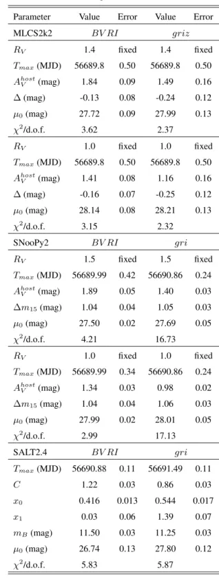
Table 6.Best-fit parameters for SN 2014J

MLCS2k2 BV RI griz

∆(mag) -0.13 0.08 -0.24 0.12

µ0(mag) 27.72 0.09 27.99 0.13

χ²/d.o.f. 3.62 2.37

∆(mag) -0.16 0.07 -0.25 0.12

µ0(mag) 28.14 0.08 28.21 0.13

χ²/d.o.f. 3.15 2.32

SNooPy2 BV RI gri

∆m15(mag) 1.04 0.04 1.05 0.03

µ0(mag) 27.50 0.02 27.69 0.05

χ²/d.o.f. 4.21 16.73

∆m15(mag) 1.04 0.04 1.06 0.03

µ0(mag) 27.99 0.02 28.01 0.05

χ²/d.o.f. 2.99 17.13

SALT2.4 BV RI gri

Tmax(MJD) 56690.88 0.11 56691.49 0.11

C 1.22 0.03 0.86 0.03

x0 0.416 0.013 0.544 0.017

x1 0.03 0.06 1.39 0.07

mB(mag) 11.50 0.03 11.25 0.03

µ0(mag) 26.74 0.13 27.80 0.12

χ²/d.o.f. 5.83 5.87

Applying SNooPy2 on their ownU BV RIJHKphotom- etry,Marion et al.(2015a) obtainedTmax(B) = 56689.74± 0.13MJD,dm15(B) = 1.11±0.02,E(B−V)host= 1.23± 0.01andµ0= 27.85±0.09mag incalibration=4mode (RV ∼1.46). Their reddening value,E(B−V)host, implies

(12)

A^host_V = 1.80±0.03mag. These parameters are marginally consistent with our results listed in Table6. However, the relatively large differences between the distance moduli obtained from the BV RI and griz data, and also between the results from MLCS2k2 and SNooPy2, suggest that the RV ∼1.4solution may not be the best one as far as LC fitting is concerned. Indeed, by comparing the distance moduli obtained from theRV ∼ 1.0 solutions, it seems that those values are more consistent with each other. The averageµ0

for the latter solution is ∼ 28.09±0.11 mag, while it is

∼ 27.72±0.20mag for theRV ∼ 1.4solution. The dispersion of the distance moduli derived from the two sets of light curves and two independent codes is much less when RV = 1.0is used for the M82 reddening law, compared to theRV ∼1.4case adopted byMarion et al.(2015a).

Fitting the combinedBV RI+g^′r^′i^′dataset with SNooPy2 gave distance moduli similar to those listed in Table6:µ⁰= 27.50±0.02(calibration=3) andµ0 = 28.02±0.02 (calibration=6). However, the reduced χ² values for the combined fits were31.66and34.79, respectively, indi- cating poor fitting quality. Comparing the best-fit template LCs with the observed ones revealed that theg^′ band data could not be fit simultaneously with the other bands: while the shape of the template LC was similar to the observed one, the observedg^′-band LC was too bright (by∼0.5mag) with respect to the template. This could be due to either an issue with our photometry (which is unlikely given that the other data do not show such a high deviation), or the complexity of the reddening law in M82 that may not be fully modeled by a singleRV (Foley et al. 2014).

The SALT2.4 code could not provide reliable distances for this heavily reddened SN. The SALT2.4 distances for SN 2014J are inconsistent with each other, as well as with the distances given by the other two codes. SALT2.4 also failed to give consistent fits to the combinedBV RI+g^′r^′i^′ LCs: neither of the templates matched the observed data ad- equately, resulting inχ²>50.

We conclude that for SN 2014J only MLCS2k2 and SNooPy2 were able to provide more-or-less consistent distances, and both of those LC fitters suggestRV ∼1.0, i.e. a lower value than found by the spectroscopic studies. How- ever, the failure of the simultaneous fitting of the combined LCs suggest that the complexity of the extinction within M82 may affect the derived distances to SN 2014J more than in the other three cases.

4.5. Correction for the host galaxy mass

The distance moduli given in Tables2-6do not contain the correction for the host galaxy mass (see Section1for references).Betoule et al.(2014) found that SNe Ia that exploded in host galaxies having total stellar mass ofMstellar >10¹⁰ M⊙are∼0.06mag brighter than those in less massive hosts.

The calibration of SALT2.4 byBetoule et al.(2014) that we applied in this paper already contains this so-called “mass- step”: theMB parameter given after Eq.3 is valid for SNe in less massive hosts, and it isMB−0.061mag for SNe in more massive hosts.

The stellar masses for the host galaxies in this paper are listed in Table1. These were derived, followingPan et al.

(2014), by applying Z-PEG⁶(Le Borgne & Rocca-Volmerange 2002) to the observed galaxy SEDs (see Table1 for references). It is seen that only SN 2014J is affected by this correction, since the hosts of the other three SNe are below logMstellar = 10. Thus, theirMBparameter does not need to be corrected, and their SALT2.4 distances are final. Un- fortunately, the SALT2.4 distance moduli of SN 2014J are unreliable as they are affected by the strong non-standard interstellar extinction (see the previous subsection). These systematic uncertainties (& 0.5 mag; Table 6) are much higher than the correction for the host galaxy mass (∼0.06 mag) in the case of SN 2014J.

Nevertheless, we investigated whether the mass-step correction could bring the derived distances to better agreement with each other for the other three SNe. Since neither MLCS2k2, nor SNooPy2 contain the mass-step correction in their calibrations, we followed the practice applied by Riess et al. (2016) by adding 0.03 mag to the MLCS2k2/SNooPy2 distance moduli of SN 2014J and sub- tracting0.03mag from the distances of SNe 2012cg, 2012ht and 2013dy, thus, mimicking the existence of the mass-step in their peak brightnesses.

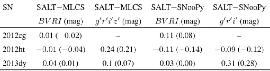
Table7shows the differences between the distance moduli estimated by SALT2.4 and the other two codes for both photometric systems after implementing the host mass correction as described above. For comparison, we give the same differences between the uncorrected distances in parentheses.

Ideally, after correction all these differences should be zero.

In reality, it is apparent that the effect of the host mass correction is minimal: sometimes it makes the agreement slightly better, sometimes slightly worse, but its amount (±0.03mag) is an order of magnitude less than the differences between the distance moduli given by the different LC-fitting codes.

It is concluded that the host mass correction on the distance modulus is negligible compared to the other sources of uncertainty, at least for the SNe studied in this paper.

Note, however, that in studies usingrelativedistances, such as Betoule et al.(2014); Riess et al.(2016) and others, this effect can be much more important and significant. There- fore, in the rest of the paper we use the uncorrected distances (i.e. without the mass-step) as given in Tables2-6, but note

6http://imacdlb.iap.fr/cgi-bin/zpeg/zpeg.pl

(13)

Table 7.Differences in distance moduli after corrections for host galaxy masses SN SALT−MLCS SALT−MLCS SALT−SNooPy SALT−SNooPy

BV RI(mag) g^′r^′i^′z^′(mag) BV RI(mag) g^′r^′i^′(mag)

2012cg 0.01 (−0.02) – 0.11 (0.08) –

2012ht −0.01(−0.04) 0.24 (0.21) −0.11(−0.14) −0.09(−0.12) 2013dy 0.04 (0.01) 0.1 (0.07) 0.03 (0.00) 0.31 (0.28) NOTE—Differences between the uncorrected distance moduli are given in parentheses.

that it is desirable to include the host mass correction in future retraining of the MLCS2k2 and/or SNooPy2 templates.

5. DISCUSSION

In this section we cross-compare the parameters derived by the three independent codes, and check the consistency between the values inferred from different photometric systems (BV RIvsgriz) and by different LC fitters.

5.1. Time of maximum light

For Type Ia SNe the moment of maximum light in theB- band has been used traditionally as the zero-point of time. At first it seems to be fairly easy to measure directly from the data, at least when the LC inB-band is available. From Ta- bles2-6it is seen that the LC fitters used in this study do a good job in estimatingTmax(B)even if theB-band LC is not included in the fitting. The consistency between the derived values is also relatively good: the dispersion around the mean values is 0.49, 0.21, 0.71 and 0.67 day for SN 2012cg, 2012ht, 2013dy and 2014J, respectively. Note, however, that SALT2.4 gets later maximum times systematically by

∆t >0.5day relative to MLCS2k2, similar to the finding by Vink´o et al.(2012) andPereira et al.(2013) for SN 2011fe.

5.2. Extinction

The host galaxy dust extinction parameters (A^host_V ) in Ta- bles 2 - 6 look generally consistent with each other. The match between the values provided by the same code for BV RI and griz is usually better than the agreement between the results of the different codes (here only MLCS2k2 and SNooPy2 are relevant, because SALT2.4 does not model dust extinction).

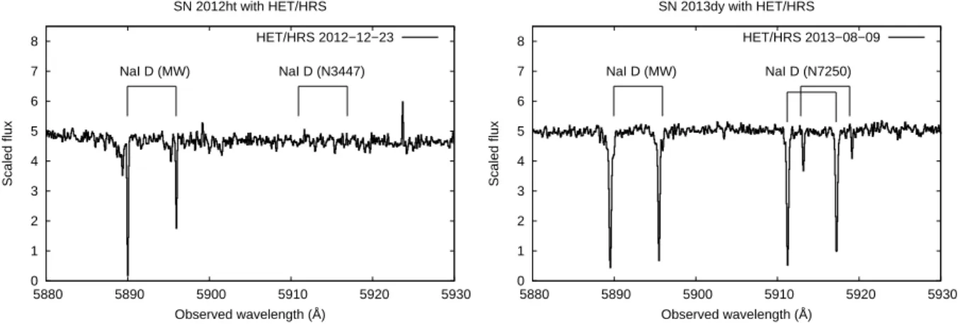
As an independent sanity check, we compare the average A^host_V values from MLCS2k2 and SNooPy2 for SN 2012ht and 2013dy with high-resolution spectra obtained with the Hobby-Eberly Telescope (HET). For SN 2013dy these spectra were published by Pan et al. (2015), while those for SN 2012ht are yet unpublished. In Fig.5the spectral regions containing the Na D (λλ5890,5896) doublet are shown. The narrow Na D features originating from the ISM both in the Milky Way and in the host galaxy (separated by the Doppler- shift due to the recession velocity of the host) are labeled.

The strength of the Na D doublet is thought to be proportional to the amount of extinction, at least as a first approximation (Richmond et al. 1994;Poznanski et al. 2012). It is seen that the dust extinction within the host galaxy for SN 2012ht is negligible (no narrow Na D absorption is visible at the redshift of the host) compared to the Milky Way component.

This is in excellent agreement with the predictions from the LC fitters, because both codes resulted inA^host_V = 0magni- tude for SN 2012ht.

Concerning SN 2013dy, the consistency between the photometric and spectroscopic extinction estimates is also very good. In Fig. 5 the Na D profiles in the host galaxy have approximately the same strength as the Milky Way components. From Tables 1 and 4, A^{M W}_V = 0.42 mag and A^host_V ∼0.44±0.14mag were taken for SN 2013dy, which are, again, in good agreement with the relative strengths of the Na D profiles in the high-resolution spectra.

The case of SN 2014J is more problematic, as this SN occured within a host galaxy that has a known complex dust content. Foley et al. (2014) presented an in-depth study of the wavelength-dependent reddening and extinction toward SN 2014J, and concluded that it is probably much more complex than a simple extinction law parametrized by a single value of AV and RV. Keeping this in mind, it is not surprising that the LC-fitting codes applied in this paper failed to produce consistent results with the spectroscopic estimates (Amanullah et al. 2014; Foley et al. 2014;

Goobar et al. 2014;Brown et al. 2015;Gao et al. 2015) that all foundRV &1.4.

5.3. Light curve shape/stretch parameter

The light curve shape/stretch parameter is the one that is most strongly connected to the peak brightness of a Type Ia SN; thus, it has a direct influence on the distance measurement. Since the three LC-fitting codes adopt slightly different parametrizations of the light curve shape, we converted each of them to the traditional ∆m15(B) (Phillips 1993). From the MLCS2k2 templates we get

∆m15(B) = 1.07 + 0.67·∆ − 0.10·∆². For SNooPy2 we adopted∆m15(B) = 0.13 + 0.89·∆m15(Burns et al.

2011), while for SALT2.4 we used∆m¹⁵(B) = 1.09− 0.161·x1+ 0.013·x²1−0.0013·x³1(Guy et al. 2007).

(14)

0 1 2 3 4 5 6 7 8

5880 5890 5900 5910 5920 5930

Scaled flux

Observed wavelength (Å) SN 2012ht with HET/HRS

NaI D (MW) NaI D (N3447)

HET/HRS 2012−12−23

0 1 2 3 4 5 6 7 8

5880 5890 5900 5910 5920 5930

Scaled flux

Observed wavelength (Å) SN 2013dy with HET/HRS

NaI D (MW) NaI D (N7250)

HET/HRS 2013−08−09

Figure 5.The narrow NaD features in the high-resolution spectrum of SN 2012ht taken at11days before maximum (left panel) and 2013dy at 12days after maximum (right panel). The components from the Milky Way and host galaxy are labeled. See text for details.

Table 8.

SN ∆m15(B) ∆m15(B) ∆m15(B)

BV RI(mag) g^′r^′i^′z^′(mag) combined (mag)

2012cg 0.984 (0.041) – –

2012ht 1.275 (0.045) 1.217 (0.041) 1.298 (0.010) 2013dy 0.960 (0.043) 0.858 (0.015) 0.971 (0.007) 2014J 1.034 (0.065) 0.952 (0.105) 0.981 (0.074) NOTE—Standard deviations are given in parentheses.

Table8lists the resulting∆m15(B)values, averaged over the three methods, for theBV RI andg^′r^′i^′z^′ data and for the combined fits, respectively. It is seen that the fits to the g^′r^′i^′z^′ data alone tend to result in systematically lower decline rates than the fits to theBV RI data or the combined BV RI+g^′r^′i^′data. The deviation is the highest in the case of SN 2013dy,∼0.1mag, and it is lower for the other two SNe.

Neglecting the differences between the other fitting parameters, an underestimate of the decline rate by∼0.1mag would cause an overestimate of∼0.08mag in the distance modulus (applying the decline rate - absolute peak magnitude calibration byBurns et al.(2014)). Since the derived distance moduli do not show such a systematic trend between theBV RI andg^′r^′i^′z^′data, and the differences between them are sometimes higher than 0.08 mag (see next section), it is concluded that the systematic underestimate of the decline rates from ourg^′r^′i^′z^′ photometry is not significant, at least from the present dataset. The number of SNe in this paper is too low to draw more definite conclusions on the cause of the depen- dence of the light curve shape/stretch parameter on the photometric bands (whether it is merely due to uncertainties in the data or might have physical origin), but it would be worth studying on a larger sample of SNe.

5.4. Distance

Distance is one of the most important outputs of the LC fitting codes under study. Cross-comparing the distance estimates produced by the various codes may reveal important constraints on the systematics that are present either in the basic assumptions of the methods or in their implementation and calibrations.

For the extremely well-observed SN 2011fe, Vink´o et al.

(2012) found a0.16±0.07mag systematic difference (∼2σ) between the distance moduli provided by MLCS2k2 and SALT2, when applied for the same homogeneous photometric data. In the left panel of Fig.6we plot the residual distance moduli (i.e. the difference of the distance modulus given by the LC-fitting code for each filter set, BV RI or griz, from the mean distance modulus) for each SNe as a function of the difference between their mean distance moduli and the ones listed in Table1. The results from fits to BV RIdata are plotted with open symbols, while those from grizdata are shown by the filled symbols. The color and the shape of the symbols encode the fitting method as indicated by the figure legend.

From this plot it is seen that a separation of ∆µ⁰ ∼ 0.2 mag can still be present between the distance moduli given by different LC-fitting codes, similar to the case of SN 2011fe, although the difference varies from SN to SN and it is less than∼ 0.2mag for the majority of the cases considered in the present paper.

For the three moderately reddened SNe (2012cg, 2012ht and 2013dy) the distances given by MLCS2k2 and SALT2.4 are in remarkable agreement (their difference is0.02,0.04 and−0.01mag, respectively) for theBV RI data. The differences between the MLCS2k2 and SNooPy2 distances in BV RIare also very good; they do not exceed0.1mag. This is not true in the case of SN 2014J, as expected, because SALT2.4 could not provide reliable distances for such an extremely reddened object, thus, they are not plotted in Fig.6.

Note that this does not mean that SALT2.4 is a less reliable