arXiv:1908.00582v1 [astro-ph.HE] 1 Aug 2019

(1)

arXiv:1908.00582v1 [astro-ph.HE] 1 Aug 2019

CONSTRAINTS ON THE PHYSICAL PROPERTIES OF TYPE IA SUPERNOVAE FROM PHOTOMETRY

R. Könyves-Tóth,¹ J. Vinkó,^{1, 2} A. Ordasi,¹ K. Sárneczky,¹ A. Bódi,^{1, 3} B. Cseh,¹G. Csörnyei,¹ Z. Dencs,¹ O. Hanyecz,¹B. Ignácz,¹Cs. Kalup,¹L. Kriskovics,¹ A. Pál,¹ B. Seli,¹ A. S´´ odor,¹ R. Szakáts,¹ P. Székely,⁴

E. Varga-Vereb´elyi,¹ K. Vida,¹ and G. Zsidi¹

1Konkoly Observatory, MTA CSFK, Konkoly-Thege M. ut 15-17, Budapest, Hungary

2Department of Optics and Quantum Electronics, University of Szeged, Hungary

3MTA CSFK Lend¨ulet Near-Field Cosmology Research Group

4Department of Experimental Physics,University of Szeged, D´om t´er 9., Szeged, Hungary

ABSTRACT

We present a photometric study of 17 Type Ia supernovae (SNe) based on multi-color (BessellBV RCIC) data taken at Piszk´estet˝o mountain station of Konkoly Observatory, Hungary between 2016 and 2018. We analyze the light curves (LCs) using the publicly available LC-fitter SNooPy2 to derive distance and reddening information. The bolometric LCs are fit with a radiation-diffusion Arnett-model to get constraints on the physical parameters of the ejecta: the optical opacity, the ejected mass and the expansion velocity in particular. We also study the pre-maximum (B−V) color evolution by comparing our data with standard delayed detonation and pulsational delayed detonation models, and show that the ⁵⁶Ni masses of the models that fit the (B−V) colors are consistent with those derived from the bolometric LC fitting. We find similar correlations between the ejecta parameters (e.g. ejecta mass, or ⁵⁶Ni mass vs decline rate) as published recently byScalzo et al.(2019).

Keywords: supenovae: general — supernovae: individual (Gaia16alq, SN 2016asf, SN 2016bln, SN 2016coj, SN 2016eoa, SN 2016ffh, SN 2016gcl, SN 2016gou, SN 2016ixb, SN 2017cts, SN 2017drh, SN 2017erp, SN 2017fgc, SN 2017fms, SN 2017hjy, SN 2017igf, SN 2018oh)

konyvestoth.reka@csfk.mta.hu

(2)

1. INTRODUCTION

Type Ia supernovae (SNe) are especially important objects for measuring extragalactic distances as their peak absolute magnitudes can be inferred via fitting their observed, multi-color LCs. Normal SN Ia events obey the empirical Phillips-relation (Pskovskii 1977; Phillips 1993), which states that the LCs of intrinsically fainter objects decline faster than those of brighter ones. The decline rate is often parametrized by ∆m15, i.e. the magnitude difference between the peak and the one measured at 15 days after maximum in a given (often the B) band. For example, the earlier version of the SNooPycode (Burns et al. 2011) applied ∆m15 as a fitting parameter for the decline rate. In the new version of SNooPy (Burns et al. 2014, 2018) a new parameter (sBV) that measures the time difference between the maxima of the B-band light curve and theB−V color curve, was introduced. Other parametrizations also exist: for example the SALT2code (Guy et al. 2007,2010;

Betoule et al. 2014) applies thex1 (stretch) parameter, whileMLCS2k2(Riess et al. 1998;Jha et al. 1999,2007) uses ∆. All of them are based on the same Phillips- relation, thus, ∆m15, sBV, x1 or ∆ are related to each other.

Studying SNe Ia opens a door for constraining the Hubble-parameter H0 (Riess et al. 2012, 2016;

Dhawan et al. 2018a) by getting accurate distances to their host galaxies. Such absolute distances are the quintessential cornerstones of the cosmic distance ladder. Via constraining H0, SNe Ia play a major role in investigating the expansion of the Universe (Riess et al. 1998; Perlmutter et al. 1999;

Astier et al. 2006; Riess et al. 2007; Wood-Vasey et al.

2007;Kessler et al. 2009;Guy et al. 2010; Conley et al.

2011;Betoule et al. 2014;Rest et al. 2014;Scolnic et al.

2014; Bengaly et al. 2015; Jones et al. 2015; Li et al.

2016; Zhang et al. 2017) and testing the most recent cosmological models (e.g. Benitez-Herrera et al. 2013;

Betoule et al. 2014).

Even though they are extensively used to estimate distances, the improvement of the precision as well as the accuracy of the method is still a subject of recent studies (see e.g. Vink´o et al. 2018). In order to achieve the desired 1% accuracy, it is important to understand the physical properties of the progenitor system and the explosion mechanism better.

The actual progenitor that explodes as a SN Ia, as well as the explosion mechanism, is still an issue. There are two main proposed progenitor scenarios: single- degenerate (SD) (Whelan & Iben 1973) and double- degenerate (DD) (Iben & Tutukov 1984). The SD scenario presumes that a carbon-oxygen white dwarf (C/O

WD) has a non-degenerate companion star, e.g. a red giant, which, after overflowing its Roche-lobe, transfers mass to the WD. When the WD approaches the Chan- drasekhar mass, spontaneous fusion of C/O to⁵⁶Ni de- velops that quickly engulfs the whole WD, leading to a thermonuclear explosion.

The details on the onset and the progress of the C/O fusion is still debated, and many possible mechanisms have been proposed in the literature. The most suc- cessful one is the delayed detonation explosion (DDE) model, in which the burning starts as a deflagration, but later it turns into a detonation wave (Nomoto et al.

1984; Khokhlov 1991; Dessart et al. 2014; Maoz et al.

2014). A variant of that is the pulsational delayed detonation explosion (PDDE): during the initial deflagration phase the expansion of the WD expels some material from its outmost layers, which pulsates, expands and avoids burning. After that, the bound material falls back to the WD that leads to a subsequent detonation (Dessart et al. 2014).

There is a theoretical possibility for a sub-Chandrasekhar double-detonation scenario, where the WD accretes a thin layer of helium onto its surface, which is com- pressed by its own mass that leads to He-detonation This triggers the thermonuclear explosion of the under- lying C/O WD (Woosley & Weaver 1994; Fink et al.

2010;Kromer et al. 2010;Sim et al. 2010,2012).

In the DD scenario two WDs merge or collide that results in a subsequent explosion (Maoz et al. 2014;

van Rossum et al. 2016).

It may be possible to distinguish between these scenarios e.g. by constraining the mass of the progenitor.

Thus, the ejecta mass is an extremely important physical quantity, which can be inferred by fitting LC models to the observations.

The idea that the bolometric LC of SNe Ia can be used to infer the ejecta mass via a semi-analytical model, was introduced by Arnett (1982) and developed further by Jeffery(1999). Arnett (1982) showed that the ejecta mass correlates with the rise time to maximum light, provided the expansion velocity and the mean optical opacity of the ejecta are known. Later, Jeffery (1999) suggested the usage of the rate of the deviation of the observed LC from the rate of the Cobalt-decay during the early nebular phase (i.e. the transparency timescale,tγ), which measures the leakage ofγ-photons from the diluting ejecta. The advantage of using tγ

for constraining the ejecta mass is that tγ is propor- tional to the gamma-ray opacity, which is much better known than the mean optical opacity. This technique was applied to real data by Stritzinger et al. (2006), Scalzo et al. (2014) and more recently by Scalzo et al.

(3)

(2019). The conclusion of all these studies was that most SNe Ia seem to have sub-Chandrasekhar mass ejecta, which was also confirmed recently by theoretical models (Dhawan et al. 2018b; Goldstein, & Kasen 2018;Wilk et al. 2018;Papadogiannakis et al. 2019).

The usage of the transparency timescale as a proxy for the ejecta mass has some caveats, though. tγ also depends on the characteristic velocity (ve) of the ex- panding ejecta, which is not easy to constrain as it is related to the velocity of a layer deep inside the ejecta.

Stritzinger et al.(2006), for example, assumed thatveis uniform for all SNe Ia (they adoptedve∼3000 km s⁻¹), which may not be true in reality, because it is known that a diversity in expansion velocities exists for most SNe Ia (Wang et al. 2013). Another issue is the distribution of the radioactive ⁵⁶Ni, encoded by the qpa- rameter by Jeffery(1999), which is usually taken from models (q ∼1/3, given by the W7 model, is often assumed). These assumptions, although may not be too far from reality, might introduce some sort of systematic uncertainties in the inferred ejecta masses, which may be worth for further studies.

The main motivation of the present paper is to give constraints on the ejecta mass and some other physical parameters for a sample of 17 recent SNe Ia (Figure 1 and 2) observed from Piszk´estet˝o station of Konkoly Observatory, Hungary. We generalize the prescription of inferring the ejecta masses by combining the LC rise time and the transparency timescale within the framework of the constant-density Arnett-model.

In the following we present the description of the photometric sample (Section 2), then we show the results from multi-color LC modeling (Section3). We construct and fit the bolometric LCs in order to derive the ejecta mass, and other parameters such as the diffusion- and gamma-leakage timescales, the optical opacity and the expansion velocity.

In Section4, we first discuss the early (de-reddened) (B−V)0color evolution, which might also provide some constraints on the explosion mechanism and the progenitor system (Hosseinzadeh et al. 2017;Miller et al. 2018;

Stritzinger et al. 2018). There is a growing number of evidence for the appearance of blue excess light during the earliest phase of some SNe Ia (Marion et al.

2016; Hosseinzadeh et al. 2017; Dimitriadis et al. 2019;

Li et al. 2018; Shappee et al. 2019; Stritzinger et al.

2018). At present the cause of this excess emission is debated, and a number of possible explanations were proposed recently (Hosseinzadeh et al. 2017; Miller et al.

2018; Stritzinger et al. 2018; Hosseinzadeh et al. 2017).

These include

• SN shock cooling;

• interaction with a non-degenerate companion;

• presence of high velocity ⁵⁶Ni in the outer layers of the ejecta;

• interaction with the circumstellar matter (CSM);

• differences in the composition or variable opacity.

Furthermore, we compare our measured (B −V)0

colors with the predictions of various explosion models (Dessart et al. 2014), and examine the possible correlations between the derived physical parameters following Scalzo et al. (2014), Scalzo et al. (2019) and Khatami & Kasen(2018).

Finally Section5summarizes the results of this paper.

2. OBSERVATIONS

We obtained multi-band photometry for 17 bright Type Ia SNe from the Piszk´estet˝o station of Konkoly Observatory, Hungary between 2016 and 2018. The se- lection criteria for the sample were as follows: i) accessi- bility from the site (i.e. declination above−15 degree), ii) sufficiently early (pre-maximum) discovery, iii) abil- ity for follow-up beyondt∼+40 days after maximum, and iv) low redshift (z.0.05).

All data were taken with the 60/90 cm Schmidt- telescope equipped with a 4096×4096 FLI CCD and Bessell BV RI filters, thus, providing a homogeneous, high signal-to-noise data sample of nearby SNe Ia.

Data reduction and photometry was done the same way as described in Vink´o et al. (2018). The raw data were reduced using IRAF¹(Image Reduction and Anal- ysis Facility) by completing bias, dark and flatfield corrections. Geometric registration of the sky frames was made in two steps. First, we used SExtractor (Bertin, E. & Arnouts, S. 1996) for identifying point sources on each frame. Second, theimwcsroutine from thewcstools² package was applied to assign R.A. and Dec. coordinates to pixels on the CCD frames.

Photometry on each SN and several other local comparison stars was made via PSF-fitting. Note that due to the strong, variable background from the host galaxy, image subtraction was unavoidable in the case of SN 2016coj, 2016gcl, 2016ixb, 2017drh and 2017hjy.

For subtraction we used template frames taken with the same telescope and instrumental setup more than 1 year after the discovery of the SN. In these cases the photometry of the comparison stars was computed on the unsubtracted frames, while it was done on the host- subtracted frames for the SN. Particular attention was

1http://iraf.noao.edu

2http://tdc-www.harvard.edu/wcstools/

(4)

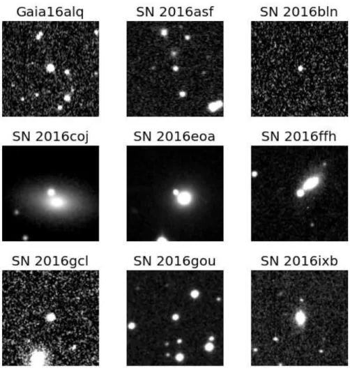
Figure 1. Images of the program SNe observed in 2016. The size of each subframe is 1.7×1.7 arcmin². The supernova is the central object, while North is up and East is to the left.

paid to keep the flux zero point of the subtracted frame the same as that of the unsubtracted one, thus, getting consistent photometry from both frames. Simple PSF fitting gave acceptable results in the case of the other SNe that suffered less severe contamination from their hosts.

The magnitudes of the local comparison stars were determined from their PS1-photometry³ after trans- forming the PS1gP, rP, iP magnitudes to the Johnson- CousinsBV RI system. The zero points of the standard transformation were tied to these magnitudes.

The basic data of the observed SNe are collected in Table 1. Plots of the V-band sub-frames centered on the SNe are shown in Fig1and2. After acceptance, all

3https://archive.stsci.edu/panstarrs/

photometric data will be made available via the Open Supernova Catalog⁴.

3. ANALYSIS

3.1. Multi-color light curve modeling

To fit and analyze the observed LCs, we used the SNooPy2⁵ (Burns et al. 2011, 2014) LC fitter, which is based on the Phillips-relation (Phillips 1993). It can be categorized as a ”distance calculator” (Conley et al.

2008), since it provides the absolute distance as a fitting parameter.

We applied both the EBV-model that fits the template LCs byPrieto et al.(2006) to the data inBV RI filters, and the EBV2-model that is based on theuBV griY JH

4https://sne.space

5http://csp.obs.carnegiescience.edu/data/snpy/snpy

(5)

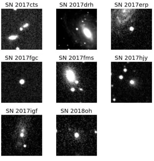
Figure 2. The same as Figure 1 but for the SNe observed in 2017 and 2018.

light curves byBurns et al.(2011). Both of these models relate the distance modulus of a normal SN Ia to its decline rate and color as

mX(ϕ) = TY +MY +µ0+KXY + +RX·E(B−V)MW +RY ·E(B−V)host, (1) where X and Y represent the filter of the template LC and the observed data,mX(ϕ) is the observed LC in filter X,TY(ϕ, p) is the template LC as a function of time, p is a generalized decline rate parameter (p = ∆m15

or p = sBV in the EBV and EBV2 models, respectively), µ0 is the reddening-free distance modulus in magnitudes, E(B−V) is the color excess due to interstellar extinction either in the Milky Way (MW), or in the host galaxy,RX,Y are the reddening slopes in filter X or Y andKXY(t, z) is the cross-band K-correction that matches the observed broad-band magnitudes of a redshifted SN taken with filter X to a template SN LC taken in filter Y. Since our SNe have very low redshifts,

K-corrections are often negligible compared to the ob- servational uncertainties (see Table1).

The motivation behind using the EBV2 model, despite the difference between the photometric system of its LC templates and our data, is that the EBV2 model allows the fitting of the sBV decline rate parameter, which is more suitable for describing fast-decliner (91bg-like) SNe Ia than the canonical ∆m15(Burns et al. 2014)⁶.

We fit the observed BV RI LCs, adoptingRV = 3.1 for the reddening slope, withχ²-minimization using the built-in MCMC routine in SNooPy2. The inferred parameters are the following:

• E(B−V)host : interstellar extinction of the host galaxy (in magnitude);

• Tmax : moment of the maximum light in the B- band (in MJD);

6We thank the referee for this suggestion.

(6)

Table 1. Basic data of the observed SNe

SN name Type R.A. Dec. Host galaxy z Discovery Ref.

Gaia16alq Ia-norm 18:12:29.36 +31:16:47.32 PSO J181229.441+311647.834 0.023 2016-04-21 a SN 2016asf Ia-norm 06:50:36.73 +31:06:45.36 KUG 0647+311 0.021 2016-03-06 b

SN 2016bln Ia-91T 13:34:45.49 +13:51:14.30 NGC 5221 0.0235 2016-04-04 c

SN 2016coj Ia-norm 12:08:06.80 +65:10:38.24 NGC 4125 0.005 2016-05-28 d

SN 2016eoa Ia-91bg 00:21:23.10 +22:26:08.30 NGC 0083 0.021 2016-08-02 e

SN 2016ffh Ia-norm 15:11:49.48 +46:15:03.22 MCG +08-28-006 0.018 2016-08-17 f

SN 2016gcl Ia-91T 23:37:56.62 +27:16:37.73 AGC 331536 0.028 2016-09-08 g

SN 2016gou Ia-norm 18:08:06.50 +25:24:31.32 PSO J180806.461+252431.916 0.016 2016-09-22 h SN 2016ixb Ia-91bg 04:54:00.04 +01:57:46.62 NPM1G +01.0158 0.028343 2016-12-17 i SN 2017cts Ia-norm 17:03:11.76 +61:27:26.06 CGCG 299-048 0.02 2017-04-02 j SN 2017drh Ia-norm 17:32:26.05 +07:03:47.52 NGC 6384 0.005554 2017-05-03 k

SN 2017erp Ia-norm 15:09:14.81 -11:20:03.20 NGC 5861 0.0062 2017-06-13 l

SN 2017fgc Ia-norm 01:20:14.44 +03:24:09.96 NGC 0474 0.008 2017-07-11 m

SN 2017fms Ia-91bg 21:20:14.60 -04:52:51.30 IC 1371 0.031 2017-07-17 n

SN 2017hjy Ia-norm 02:36:02.56 +43:28:19.51 PSO J023602.146+432817.771 0.007 2017-10-14 o

SN 2017igf Ia-91bg 11:42:49.85 +77:22:12.94 NGC 3901 0.006 2017-11-18 p

SN 2018oh Ia-norm 09:06:39.54 +19:20:17.77 UGC 04780 0.012 2018-02-04 q

Note—a: Piascik, & Steele(2016); b: Cruz et al.(2016); c: Miller et al.(2016); d: Zheng et al.(2017); e: Gagliano et al.

(2016); f: Tonry et al.(2016); g: Brown(2016); h: Tonry et al.(2016); i: Stanek(2016); j: Brimacombe et al.(2017); k:

Valenti et al.(2017); l: Itagaki(2017); m: Sand et al.(2017); n: Gagliano et al.(2017); o: Tonry et al.(2017); p: Stanek (2017); q:Stanek(2018)

• µ0 : extinction-free distance modulus (in magnitude);

• sBV: decline rate parameter in the EBV2 model

• ∆m15 : decline rate parameter in the EBV model (in magnitude).

We also attempted to includeRV as a fitting parameter, but the results were close the original RV = 3.1 value, indicating that our photometry is not suitable for constraining this parameter. This is not surprising, given the lack of UV- or NIR-data in our sample.

Note that since the EBV2 model is based on a different photometric system than our Johnson-Cousins BV RI data, the inferred best-fit values for E(B−V) andµ0

are expected to be slightly different from those obtained from the EBV model that is based onBV RIdata. After comparing the best-fit parameters taken from both models, it is found that the E(B−V) values are consistent with each other within 1σ, while there is a systematic shift of µ0(EBV)−µ0(EBV2)∼0.1 mag between the distance moduli. For consistency, we decided to adopt theE(B−V) andµ0parameters from the EBV2 model as final, but added ∼ 0.1 mag systematic uncertainty

to the distance modulus (corresponding to ∼5 percent relative error in the distances).

The final best-fit parameters are shown in Table 2.

The reported errors include the systematic uncertainties of the template vectors as given bySNooPy2.

Plots of the observed LCs and their best-fit SNooPy2 templates can be found in the Appendix (Fig. 11). The overall fitting quality is good; most of the reduced χ² values (column 8 in Table 2) are in between 1 and 2, and the highestχ² ∼6.6 is that of SN 2016gou. As it can be seen in Fig. 11, the fit to SN 2016gou around maximum is very good, and the relatively highχ²value is likely caused by the scattering in the last few data points after +40 days.

As seen in Table2, the host reddening of SN 2017drh turned out to be extremely high (E(B −V)host ∼ 1.4 mag) compared to the rest of the sample. Since this may add an extra uncertainty in the derived distance and other parameters, SN 2017drh was excluded from the sample and was not analyzed further.

3.2. Construction of the bolometric light curve While constructing the bolometric LCs we followed the same procedure as applied recently by Li et al.

(7)

0 0.1 0.2 0.3 0.4 0.5

0 10 20 30 40 50

fBUV / fbol

Days since explosion 2018oh Swift

2018oh estimate 2011fe Swift 2011fe estimate 2017erp Swift 2017erp estimate

0.001 0.01 0.1 1

0 20 40 60 80 100

Luminosity (1043 erg s−1)

Days since explosion

BVRI extended UV+BVRI+IR

0.0001 0.001 0.01 0.1 1

0 20 40 60 80 100 UV estimate

0.001 0.01 0.1 1

0 20 40 60 80 100 IR estimate

0.1 0.15 0.2 0.25 0.3 0.35 0.4 0.45

-20 -10 0 10 20 30

fBUV / fbol

Days since B-maximum Ia-normal

Ia-91T Ia-91bg 2011fe

0 5x10⁴² 1x10⁴³ 1.5x10⁴³ 2x10⁴³ 2.5x10⁴³

-20 -10 0 10 20 30 40 50 60 70 80

L (erg/s)

Days since B-maximum 16alq 16asf 16coj 16ffh 16gou 17cts 17drh 17erp 17fgc 17hjy 18oh 16bln 16gcl 16ixb 16eoa 17fms 17igf 11fe

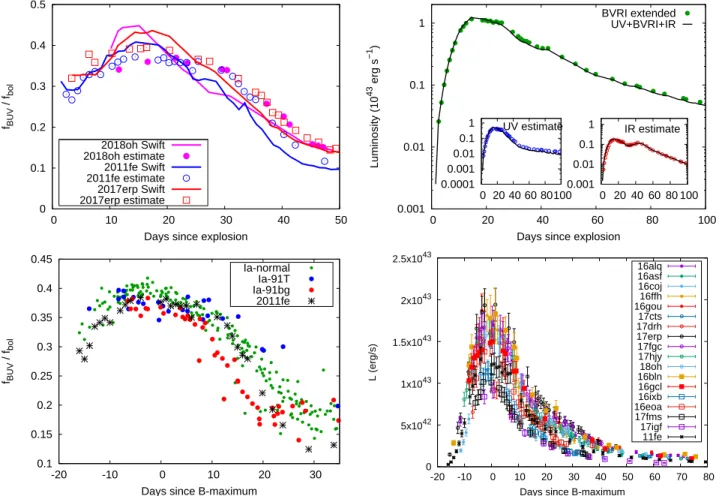
Figure 3. Top left panel: the ratio of BUV flux to the total bolometric flux as a function of time since explosion for SN 2018oh (magenta), SN 2011fe (blue) and SN 2017erp (red). Data obtained by direct integration ofSwiftfluxes are plotted with lines, while the symbols correspond to data estimated fromBVRIobservations (see text). Top right panel: Comparison of the pseudo- bolometric LCs of SN 2011fe derived from the extrapolatedBV RISED (symbols) and by direct integration of the observed UV + optical + NIR data (black line). The two insets show the UV and the IR contributions separately. Bottom left panel: the same as the top left panel but for the whole observed sample. Colors code the different SN subtypes as indicated in the legend.

Bottom right panel: the derived pseudo-bolometric light curves for the sample SNe.

(2018) for SN 2018oh. Briefly, after correcting for extinction within the Milky Way and the host galaxy (Table 1 and 2), the observed BV RI magnitudes were converted to physical fluxes via the calibration of Bessell et al. (1998). Then, the fluxes were integrated against wavelength via the trapezoidal rule. The missing UV- and IR bands are estimated by extrapolations in the following way.

In the UV regime the flux was assumed to decrease lin- early between 2000 ˚A andλB, and the UV-contribution was estimated from the extinction-correctedB-band flux fB asf_bol^UV = 0.5fB(λB−2000).

In the IR, a Rayleigh-Jeans tail was fit to the corrected I-band flux fI and integrated between λI and infinity to getf_bol^IR = 1.3fIλI/3. The factor 1.3 was applied to match the extrapolated IR-contribution to the

pseudo-bolometric fluxes obtained via direct integration of observed near-IRJHK photometry (see below).

Finally, the bolometric fluxes are corrected for distances using the distance moduli taken from the SNooPy2fits (Section3.1).

This procedure was validated by comparing the estimated UV and IR-contributions to those calculated from existing data for three well-observed normal Type Ia SNe: 2011fe (Brown et al. 2014; Vink´o et al. 2012;

Matheson et al. 2012), 2017erp (Brown et al. 2018) and 2018oh (Li et al. 2018). All data were downloaded from theOpen Supernova Catalog⁷ (Guillochon et al. 2017).

Fig.3shows the comparison of theBV RI-extrapolated pseudo-bolometric fluxes (colored symbols) with the

7https://sne.space

(8)

Table 2. Best-fit parameter from SNooPy2

Name E(B−V)M W E(B−V)host Tmax µ0 sBV ∆m15 χ²

mag mag MJD mag mag

SN 2011fe 0.0075 0.048 (0.060) 55815.31 (0.06) 29.08 (0.082) 0.940 (0.031) 1.175 (0.008) 1.058 Gaia16alq 0.0576 0.089 (0.061) 57508.11 (0.14) 35.05 (0.084) 1.132 (0.033) 0.939 (0.024) 1.358 SN 2016asf 0.1149 0.076 (0.097) 57464.66 (0.11) 34.69 (0.083) 1.001 (0.031) 1.102 (0.023) 2.722 SN 2016bln 0.0249 0.213 (0.061) 57499.40 (0.34) 34.78 (0.116) 1.058 (0.032) 1.005 (0.024) 3.839 SN 2016coj 0.0163 0.000 (0.061) 57548.30 (0.34) 32.08 (0.083) 0.788 (0.030) 1.438 (0.020) 1.954 SN 2016eoa 0.0633 0.242 (0.062) 57615.66 (0.35) 34.24 (0.101) 0.775 (0.032) 1.486 (0.036) 1.867 SN 2016ffh 0.0239 0.198 (0.061) 57630.48 (0.36) 34.61 (0.094) 0.926 (0.032) 1.082 (0.018) 2.392 SN 2016gcl 0.0630 0.056 (0.061) 57649.48 (0.36) 35.45 (0.090) 1.155 (0.043) 0.901 (0.031) 2.792 SN 2016gou 0.1095 0.258 (0.060) 57666.40 (0.34) 34.25 (0.104) 0.984 (0.031) 0.925 (0.032) 6.560 SN 2016ixb 0.0520 0.077 (0.061) 57745.11 (0.37) 35.620 (0.087) 0.758 (0.032) 1.657 (0.039) 2.072 SN 2017cts 0.0265 0.158 (0.061) 57856.83 (0.35) 34.56 (0.088) 0.931 (0.030) 1.208 (0.020) 1.394 SN 2017drh 0.1090 1.396 (0.062) 57890.94 (0.36) 32.29 (0.326) 0.838 (0.031) 1.352 (0.065) 2.075 SN 2017erp 0.0928 0.210 (0.061) 57934.40 (0.35) 32.34 (0.097) 1.174 (0.030) 1.129 (0.011) 1.627 SN 2017fgc 0.0294 0.162 (0.061) 57959.77 (0.37) 32.61 (0.092) 1.137 (0.037) 1.086 (0.027) 1.761 SN 2017fms 0.0568 0.022 (0.061) 57960.09 (0.35) 35.52 (0.084) 0.746 (0.033) 1.425 (0.026) 1.875 SN 2017hjy 0.0768 0.211 (0.061) 58056.02 (0.35) 34.05 (0.096) 0.949 (0.031) 1.137 (0.011) 1.519 SN 2017igf 0.0456 0.158 (0.061) 58084.61 (0.36) 32.80 (0.096) 0.608 (0.032) 1.757 (0.006) 3.461 SN 2018oh 0.0382 0.071 (0.061) 58162.96 (0.37) 33.40 (0.083) 1.089 (0.034) 0.989 (0.013) 1.231

(9)

ones obtained by direct integrations from the UV to the NIR. In the latter case, the integral of a Rayleigh-Jeans tail was also added to the final bolometric flux, but the tail was fit to the K-band flux (fK) instead offI and the factor 1.3 was not applied.

The top-left panel exhibits the comparison of the flux ratiofBUV to fbol as a function of phase, where fBUV

is the integrated flux between the B-band and 2000 ˚A and fbol is the total bolometric flux. The filled circles are based on interpolated fluxes (as described above), while the lines are from direct integration using the UV data from theNeil Gehrels Swift Observatorydatabase.

It is seen that there is reasonable agreement between the interpolated and the directly integrated blue-UV fluxes.

The bottom-left panel shows the same flux ratio computed from the interpolated data but for all SNe in our sample. This illustrate that there is no major difference in the flux ratios between the slow- and fast-decliner SNe Ia around maximum light, despite a ∼ 5 percent relative flux uncertainty (estimated from the scattering of the data) that we include in the final flux uncertainty estimate.

In the top-right panel the full bolometric LC from direct integration (solid line) and the one based on extrap- olation (circles) is shown for the extremely well-observed SN 2011fe. The insets illustrate the same but only for the UV (left) and NIR (right) regimes. Again, there seems to be good agreement between the directly integrated and the extrapolated bolometric fluxes. In the bottom-right panel the calculated luminosity evolution is plotted for all SNe in our sample.

It is concluded that the pseudo-bolometric LCs obtained from extrapolations described above are reliable representations of the true bolometric data, and the systematic errors due to the missing bands do not exceed

∼5 percent. Together with the errors due to uncertainties in the distances (see above), the final relative uncertainty of the bolometric fluxes are estimated as∼10 percent.

3.3. Fitting the bolometric light curve

We estimated the physical parameters of the SN ejecta via applying the radiation-diffusion model of Arnett (1982), fitting the bolometric LCs with theMinimcode (Chatzopoulos et al. 2013). This is a Monte-Carlo code utilizing the Price-algorithm that intends to find the po- sition of the absolute minimum on the χ²-hypersurface within the allowed volume of the parameter space. Pa- rameter uncertainties are estimated from the final distribution ofN = 200 test points that probe the parameter space around the χ² minimum where ∆χ² ≤ 1. See Chatzopoulos et al.(2013) for more details.

The fitted parameters were the following: the time of the first light (t0), the light curve time scale (tlc), the gamma-ray leaking time scale (tγ), and the initial nickel mass (MN i). These parameters can be found in Table 3. The final uncertainty of the nickel mass also contains the error of the distance (as given by SNooPy2) which is added to the fitting uncertainty reported byMinimin quadrature. Figure12in the Appendix shows the best- fit bolometric LCs corresponding to the smallestχ².

The crucial parameter in the semi-analytic LC codes is the effective optical opacity (κ) that is assumed to be constant both in space and time. To estimate the effective optical opacity for our sample, we applied the same technique as done byLi et al.(2018) for SN 2018oh recently. This technique is based on the combination of the light curve time scale,tlcand that of the gamma-ray leakage,tγ. These parameters can be expressed with the physical parameters of the ejecta as follows

t²_lc = 2κMej

βcvexp

and t²_γ = 3κγMej

4πv²_exp (2) where Mej is the ejecta mass, β = 13.8 is a fixed LC parameter related to the density distribution, vexp is the expansion velocity and κγ = 0.03 cm²g⁻¹ is the opacity forγ-rays (Arnett 1982;Clocchiatti & Wheeler 1997; Valenti et al. 2008; Chatzopoulos et al. 2012;

Wheeler et al. 2015;Li et al. 2018).

Since tlc andtγ are measured quantities, the two for- mulae in Equation 2 contains three unknowns: Mej, vexp, and κ. Following Li et al. (2018), we apply two additional constraints for Mej and vexp to get upper and lower limits for κ. Assuming that the ejecta mass cannot exceed the Chandrasekhar limit (Mej ≤ MCh) we get a lower limit for the optical opacity, κ⁻, while assuming a lower limit forvexpasvexp≥10,000 km s⁻¹ we get an upper limit,κ⁺ (see Equation2.).

In the first case the lower limit forκcan be calculated as

κ⁻ =

s 3κγt⁴_lcβ²c²

16πt²_γMCh. (3) Second, the lower limit for the expansion velocity, vexp= 10,000 km s⁻¹, implies

κ⁺ = 3κγt²_lcβc

8πvexpt²_γ. (4) The inferred κ and κ⁺ values can be found in Table 3.

Finally we estimateκas the average ofκandκ⁺, and deriveMej andvexpvia the following expressions

Mej = 3κγt⁴_lcβ²c²

16πt²_γκ² and vexp = 3κγt²_lcβc 8πκt²_γ . (5)

(10)

Table 3.Best-fit and inferred parameters from the bolometric LC fitting

Name t0 t_lc tγ MN i κ⁻ κ⁺ Mej vexp E_kin χ²

(day) (day) (day) (M⊙) (cm²g⁻¹) (M⊙) (km s⁻¹) (10⁵¹erg)

2011fe 16.59 (0.061) 14.87 (0.321) 37.60 (0.670) 0.567 (0.042) 0.166 0.232 1.002 (0.070) 11660 (542) 0.817 (0.407) 0.517 Gaia16alq 19.92 (0.418) 13.78 (0.899) 46.669 (0.717) 0.744 (0.055) 0.115 0.129 1.274 (0.330) 10594 (1421) 0.858 (0.269) 1.755 2016asf 15.08 (2.579) 11.35 (1.140) 39.192 (1.329) 0.597 (0.149) 0.093 0.124 1.051 (0.430) 11459 (2429) 0.828 (0.491) 0.502 2016bln 17.42 (0.342) 14.00 (1.219) 44.508 (1.125) 0.789 (0.097) 0.124 0.146 1.211 (0.430) 10833 (1964) 0.852 (0.363) 0.662 2016coj 14.17 (0.261) 10.57 (0.367) 32.967 (0.863) 0.401 (0.053) 0.095 0.152 0.856 (0.130) 12298 (1070) 0.777 (0.557) 0.487 2016eoa 14.07 (3.053) 10.55 (1.092) 39.038 (0.935) 0.482 (0.103) 0.080 0.108 1.047 (0.440) 11483 (2439) 0.828 (0.498) 0.617 2016ffh 14.03 (1.16) 9.736 (0.521) 40.521 (0.926) 0.573 (0.078) 0.067 0.088 1.035 (0.230) 11298 (1316) 0.836 (0.363) 0.653 2016gcl 17.79 (2.184) 15.85 (1.177) 43.623 (1.182) 0.689 (0.164) 0.162 0.195 1.185 (0.360) 10931 (1728) 0.849 (0.343) 0.280 2016gou 15.03 (0.525) 11.05 (0.798) 45.793 (1.412) 0.678 (0.063) 0.075 0.086 1.250 (0.30) 10696 (1681) 0.856 (0.304) 0.263 2016ixb 15.64 (2.088) 13.12 (2.364) 30.520 (1.345) 0.483 (0.064) 0.159 0.274 0.777 (0.30) 12653 (3050) 0.747 (0.539) 0.177 2017cts 14.23 (1.101) 9.97 (1.259) 42.485 (0.959) 0.539 (0.063) 0.066 0.081 1.151 (0.58) 11062 (2838) 0.845 (0.505) 0.506 2017erp 17.96 (0.092) 17.40 (0.518) 37.603 (1.084) 0.975 (0.083) 0.227 0.317 1.002 (0.13) 11661 (966) 0.817 (0.414) 0.413 2017fgc 16.21 (0.239) 12.50 (0.386) 45.398 (0.941) 0.692 (0.047) 0.097 0.112 1.237 (0.16) 10734 (799) 0.855 (0.210) 0.253 2017fms 14.04 (0.504) 10.58 (0.575) 34.612 (0.731) 0.360 (0.029) 0.091 0.138 0.909 (0.20) 12066 (1407) 0.794 (0.523) 0.264 2017hjy 16.29 (0.492) 12.83 (0.823) 39.484 (0.840) 0.688 (0.057) 0.117 0.156 1.060 (0.270) 11425 (1545) 0.830 (0.406) 0.213 2017igf 19.58 (0.933) 15.30 (1.353) 34.554 (1.193) 0.420 (0.051) 0.191 0.291 0.906 (0.320) 12070 (2291) 0.792 (0.572) 0.779 2018oh 14.86 (0.864) 11.17 (1.098) 44.654 (0.928) 0.598 (0.059) 0.078 0.092 1.217 (0.480) 10824 (2175) 0.856 (0.394) 0.187

HavingMejandvexpevaluated, we express the kinetic energy of ejecta asEkin= 0.3·Mej·v_exp² (Arnett 1982;

Chatzopoulos et al. 2012).

The results of these calculations are collected in Ta- ble 3, where the uncertainties (given in parentheses, as previously) are calculated via error propagation taking into account the uncertainties of the fitted timescales and the mean optical opacity, the latter approximated as ∆κ≈0.5(κ⁺−κ⁻).

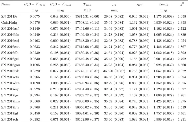
In order to illustrate that the ejecta mass can be inferred from the combination of tlc and tγ via Eq. 5, we constructed model LCs with different ejecta parameters. The left panel of Fig.4 shows some of them corresponding to κ= 0.1 cm²g⁻¹, vexp = 11,000 km s⁻¹, and Mej in between 0.5 and 2.1 M⊙. It can be seen that largerMej implies both longer rise time and slower decline rate consistently with Eq. 2. The right panel indicates the correlation between the ejecta mass and the two time scale parameters,tlcandtγ. Heretγ is plotted with squares while tlc with triangles, and different colors code different physical parameters as follows: blue means vexp = 11,000 km s⁻¹, κ = 0.1 cm²g⁻¹, green denotes vexp = 15,000 km s⁻¹, κ = 0.1 cm²g⁻¹, and orange is vexp = 11,000 km s⁻¹, κ = 0.2 cm²g⁻¹. As it is expected, the shorter the time scales, the lower the model ejecta mass, suggesting that the combination of tlc and tγ outlined above may indeed provide realistic estimates forMej.

We use two SNe as reference objects in order to test the consistency of our LC modeling described above with those presented in other studies. SN 2011fe is chosen as the first test object due to the availability of precise,

high-cadence observations spanning from the near-UV to the near-IR regimes (see Section 3.2). Scalzo et al.

(2014) modeled the bolometric LC of SN 2011fe and obtained Mej = 1.19±0.12 M⊙ and MN i = 0.42±0.08 M⊙ for the ejected mass and the nickel mass, respectively. Our best-fit results are Mej = 1.00 ±0.070 M⊙ and MN i = 0.567±0.042 M⊙ (see Table 3). It is seen that these two estimates are only marginally consistent: the difference between the two ejecta masses ex- ceeds 1σslightly, while the ⁵⁶N i-masses differ by∼2σ.

In addition to the sensitivity of the ⁵⁶N i-mass to the uncertainties in the distance, this highlights the possible systematic differences between the two modeling schemes applied by Scalzo et al. (2014) and in this paper: Scalzo et al. (2014) used only the late-time bolometric LC to constrain the ejecta and nickel masses viatγ based on the method of Jeffery(1999), while we fit the full Arnett-model to the entire LC. Note that the ⁵⁶N i mass of SN 2011fe has also been determined in several other papers, including Pereira et al. (2013) (0.53 ±0.11 M⊙), Mazzali et al. (2015) (0.47±0.07 M⊙) and Zhang et al. (2016) (0.57 M⊙). The scattering of these various estimates suggest a value of MN i ∼0.5±0.1 M⊙ for SN 2011fe, which makes both our result and that ofScalzo et al.(2014) consistent.

On the other hand, good agreement is found between the parameters of the other test object, SN 2018oh. Re- cently Li et al. (2018) derived Mej = 1.27±0.15 M⊙

and MN i = 0.55 M⊙, which are very similar to our best-fit values (Table 3), Mej = 1.22±0.48 M⊙ and MN i = 0.60±0.06 M⊙. Even though Li et al. (2018) applied the same method for the LC fitting as we use in

(11)

0 0.5 1 1.5 2 2.5

0 10 20 30 40 50 60 70 80 90 100 Lbol (1043 erg s−1)

Days since explosion

0.5 M_o 0.7 M_o 0.9 M_o 1.1 M_o 1.3 M_o 1.5 M_o 1.7 M_o 1.9 M_o 2.1 M_o

0 10 20 30 40 50 60

0.4 0.6 0.8 1 1.2 1.4 1.6 1.8 2 2.2

Time scales (days)

M_ej (M_o)

t_lc t_γ

Figure 4. Left panel: bolometric LCs for models havingMej in between 0.5 and 2.1 M⊙. All other input parameters for the models were fixed asR0 = 0.01R⊙,vexp= 11 000 km s⁻¹,κ= 0.1 cm²g⁻¹, andMN i = 0.6 M⊙. Right panel: tlc (triangles) andtγ (squares) as a function ofMej. The values corresponding tovexp= 11000 km s⁻¹ andκ= 0.1 cm²g⁻¹ are plotted with blue,vexp= 15000 km s⁻¹ andκ= 0.1 cm²g⁻¹with green, andvexp= 11000 km/s,κ= 0.2 cm²g⁻¹ with orange symbols.

this paper, their bolometric LC was assembled from a much denser, more extended dataset, including observed near-UV and near-IR photometry. The good agreement between our best-fit parameters and theirs suggests that our parameters are not unrealistic, and probably do not suffer from severe systematic errors.

4. DISCUSSION 4.1. Early color evolution

In Fig.5we plot the early (B−V)0 colors, corrected for both Milky Way and host galaxy reddening (Table 2), of our sample together with the data for several other well-observed SNe Ia: SN 2017cbv (Hosseinzadeh et al.

2017), SN 2011fe (Vinkó et al. 2012), SN 20112cg (Vinkó et al. 2018), SN 2017fr (Contreras et al. 2018), SN 2009ig (Marion et al. 2016; Foley et al. 2012), iPTF16abc (Miller et al. 2018), SN 2012ht (Vinkó et al.

2018) and SN 2013dy (Vink´o et al. 2018)). In the following we investigate the pre-maximum color evolution of our observed sample.

Early-phase (B−V)0 observations of SNe Ia suggest that they can be divided into two categories: early- red and early-blue type (e.g. Stritzinger et al. 2018).

The cause of this dichotomy is still debated (see Sec- tion1). For example,Miller et al.(2018) proposed physical models for the progenitor system and the explosion of iPTF16abc. This SN Ia showed blue, nearly constant (B−V)0 color starting from t ∼-10 days, which was thought to be caused by strong⁵⁶Ni-mixing in the ejecta.

SNe Ia experience a dark phase after shock breakout (SB), before the heating from radioactive decay diffuses through the photosphere. The duration of this dark

phase depends on how much⁵⁶Ni is mixed into the outer layers of the ejecta. If⁵⁶Ni is confined to the innermost layers, the dark phase lasts for a few days, so that weak mixing leads to redder colors and moderate luminosity rise. On the contrary, strong mixing results in higher luminosities and bluer optical colors. In the latter case the dark phase does not exist or very short, because the γ-photons originating from the Ni-decay rapidly diffuse out from the ejecta. Shappee et al. (2019) found that strong mixing accounts for the early excess light in the LC of SN 2018oh observed byKeplerduring the K2-C16 campaign, although its color could not be constrained by the unfiltered K2 observations.

Another possibility for the early blue flux is the collision of the ejecta into a nearby companion star or some kind of a circumstellar envelope. In this case a strong, quickly declining ultraviolet pulse is thought to be the root cause of the excess blue emission during the earliest phases. However, the observability of this emission re- quires a favorable geometric configuration, i.e. the companion being in front of the SN toward the observer, so it is expected to occur in less than 10% of the actually observed SNe Ia (e.g.Kasen 2010).

With the use of our new photometric data we attempt to investigate the evolution of the early (B−V)0 color for our sample SNe Ia. Fig.5 illustrates that our data are consistent with the colors of other SNe Ia collected from recent literature (plotted as continuous lines in the left panel of Fig. 5) as well as those computed from the Hsiao-template (Hsiao et al. 2007) shown with a black line in both panels. In the latter case the colors are derived by synthetic photometry using BessellB andV

(12)

-0.8 -0.6 -0.4 -0.2 0 0.2 0.4 0.6

-20 -15 -10 -5 0

(B-V)0

Rest-frame days

2017cbv 2011fe 2012cg 2012fr 2009ig 2016abc 2012ht 2013dy 16alq 16asf 16coj 16ffh 16gou 17cts 17drh 17erp 17fgc 17hjy 18oh 16bln 16gcl 16ixb 16eoa 17fms 17igf

-1 -0.5 0 0.5 1 1.5 2 2.5

-20 0 20 40 60 80

(B-V)0

Rest-frame days

16alq 16asf 16coj 16ffh 16gou 17cts 17drh 17erp 17fgc 17hjy 18oh 16bln 16gcl 16ixb 16eoa 17fms 17igf Hsiao

Figure 5. The evolution of the reddening-corrected (B−V)0 colors for the sample SNe (colored symbols). Left panel: the pre-maximum color evolution compared to other well-observed SNe collected from literature (colored lines). Right panel: B−V0

colors of the sample plotted together with Hsiao template (green curve) up to 90 days after maximum.

filter functions (Bessell 1990) on the spectral templates ofHsiao et al.(2007).

In order to classify SNe Ia into the early-red and early- blue groups, photometric data taken between −20 and

−10 days before maximum is necessary. Between t =

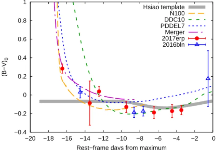
−10 days and tmax the (B−V)0 colors are so similar for most SNe Ia that it is almost impossible to make such a distinction. Unfortunately, most of the SNe Ia in our sample do not have photometry taken early enough for this purpose. During our campaign this very early phase (−20< t <−10 days) have been observed only in two cases: SN 2016bln and 2017erp (see the left panel in Figure5).

SN 2016bln, a 1991T-like or slow-decliner Ia belonging to the Type SS (Shallow Silicon) subclass on the Branch- diagram (Cenko et al. 2016), shows a very blue early (B−V)0 color in Fig. 5. It suggests that SN 2016bln may be associated with the early-blue group. This is consistent with the findings of Stritzinger et al. (2018) who showed that SNe having early blue colors tend to be located in between the Core Normal and the Shal- low Silicon types in the Branch diagram, similar to the 1991T-like events.

On the other hand, SN 2017erp has an early (B − V)0 color that is similar to that of SN 2011fe, thus, it belongs to the early-red group. It is interesting that Brown et al.(2018) showed that SN 2017erp was a near- UV (NUV)-red object, while SN 2011fe was a NUV-blue event. This difference between the NUV-colors seems to be independent from the early-phase optical colors, because 2011fe and 2017erp both had similarly red early (B−V)0 color.

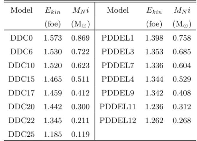
Table 4. Parameters of the DDE and PDDE models by Dessart et al.(2014)

Model Ekin MNi Model Ekin MNi

(foe) (M⊙) (foe) (M⊙)

DDC0 1.573 0.869 PDDEL1 1.398 0.758 DDC6 1.530 0.722 PDDEL3 1.353 0.685 DDC10 1.520 0.623 PDDEL7 1.336 0.604 DDC15 1.465 0.511 PDDEL4 1.344 0.529 DDC17 1.459 0.412 PDDEL9 1.342 0.408 DDC20 1.442 0.300 PDDEL11 1.236 0.312 DDC22 1.345 0.211 PDDEL12 1.262 0.268 DDC25 1.185 0.119

This result may suggest that the observed spread in the early NUV- and optical (B −V) colors of SNe Ia has different physical reasons. Brown et al.(2018) concluded that the diversity in the NUV colors is likely due to the metallicity of the progenitor that affects the NUV-continuum and the strength of the Ca H&K fea- tures. The fact that SN 2017erp and SN 2011fe have similar early (B −V)0 but different NUV colors may suggest that the early (B−V)0 diversity might not be directly related to the progenitor metallicity.

4.2. Comparison with explosion models

In this subsection we compare parameters derived from the bolometric LC fitting, in particular the nickel mass, to those taken from several explosion models.

First, we consider the DDE and PDDE models computed byDessart et al.(2014), as listed in Table4. It is

(13)

0.1 0.2 0.3 0.4 0.5 0.6 0.7 0.8 0.9 1 1.1

0.3 0.4 0.5 0.6 0.7 0.8 0.9 1 1.1 MNi (model)

M_Ni (bol)

DDE models PDDE models

Figure 6. Comparison of the Ni-masses derived from the bolometric LCs (plotted on the horizontal axis) with those from DDE (red symbols) and PDDE (blue symbols) models (vertical axis). Solid line represents the expected 1:1 relation.

seen that the Ni-masses of these models span the same range than the ones inferred from the bolometric LC fitting (see Table3), but the kinetic energies of the models are higher by about a factor of ∼2.

PDDE models exhibit strong C II lines shortly after explosion, which are formed in the outer, unburned material. Furthermore, the collision with the previously ejected unbound material surrounding the WD results in the heat-up of the outer layers of the ejecta. Thus, in the PDDE scenario the early color of the SN is bluer, and the luminosity rises faster than in the conventional DDE models.

On the contrary, standard DDE models typically leave no unburned material. Instead, at 1-2 days after explosion they show red optical colors ((B−V)0∼1 mag ), which gets bluer continuously as the SN evolves toward maximum light. After maximum both the DDE and the PDDE scenarios show nearly the sameB−V color.

We compare the observed, reddening-corrected (B− V)0colors of our sample with the predictions from these explosion models. The colors from the models were derived via synthetic photometry applying the standard Bessell B and V filters (Bessell 1990), as above.

Note that the in the redshift range of the observed SNe (z≤0.031) the K-corrections for the (B−V) color in- dices does not exceed 0.06 mag, which is comparable to the uncertainty of our color measurements in these bands. Thus, the K-corrections were neglected when computing the observed (B−V)0colors for the comparison with the explosion models. A plot comparing the color curves inferred from DDE and PDDE models with the observed ones can be found in Figures 13and14in the Appendix.

−0.4

−0.2 0 0.2 0.4 0.6 0.8 1

−20 −18 −16 −14 −12 −10 −8 −6 −4 −2 0

(B−V)0

Rest−frame days from maximum Hsiao template

N100 DDC10 PDDEL7 Merger 2017erp 2016bln

Figure 7. Comparison of the early (dereddened) (B−V)0

colors of SN 2017erp (red circles) and 2016bln (blue triangles) with the ones predicted by several Ia explosion models (DDE, PDDE and Violent Merger mechanisms, see text).

The color evolution from the empirical Hsiao template is also shown with a thick grey line.

After computing the syntheticB−V curves as a function of phase, the one that has the lowest χ² with re- spect to the observed (B−V)0 color curve was chosen as the most probable explosion model that describes the observed SN. Figure6 compares the Ni-masses of these models to those derived directly from bolometric LC fitting (Table3).

Although the grid resolution of the models is inferior, it is seen that the nickel masses from the DDE models nicely correlate with the ones from the bolometric LC fitting (the only outlier, SN 2017erp, may have an over- estimatedMN i∼1 M⊙ due to a reddening issue). The agreement is worse for the PDDE models, where most of the best-fit models have practically the same Ni-mass, MN i∼0.6 - 0.7 M⊙.

In Figure7a similar comparison of the syntheticB−V colors from different explosion models with observations is shown, but only for the pre-maximum phases. Beside two models considered above (DDC10 and PDDEL7) byDessart et al.(2014), synthetic colors from two other theoretical models are also plotted: the N100 explosion model (DDE in a Chandrasekhar-mass WD) by Seitenzahl et al. (2013) and the Violent Merger (VM) model by Pakmor et al. (2012). The color evolution from the empirical Hsiao template (Hsiao et al. 2007) is also shown for comparison.

It is seen that three of these models (N100, PDDEL17 and VM) show similar pre-maximumB−V colors than the observations even at the earliest (t < −14 days) phases. The DDC10 model byDessart et al.(2014) pre- dicts too redB−V color at the earliest phases, while

(14)

the colors from the Hsiao template look being too blue.

Although the models shown here do not seem to constrain the observed early-blue and early-red events, at least the two SNe in our sample (2016bln and 2017erp) that have been sampled att <−14d haveB−V colors consistent with the first three models.

It is concluded that the observedB−V color evolution of SNe Ia seems to be more-or-less reproduced by current models of DDE and/or VM mechanisms. The Ni-masses of the DDE models byDessart et al.(2014) that match the observed B−V colors are consistent with the Ni- masses inferred from the bolometric LC fitting. This is not true for the PDDE models, as they predict too high nickel masses for SNe that have MN i < 0.6 M⊙ from their bolometric LC fitting.

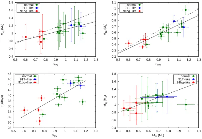
4.3. Ejecta parameters

In this section we examine the relations between the inferred ejecta parameters (Table 3) following Scalzo et al. (2014) and Scalzo et al. (2019). Overall, we find similar correlations between the ejecta mass, the Ni-mass and the LC timescales (tcl,tγ, andsBV) to those presented recently byScalzo et al.(2019).

4.3.1. Comparison withScalzo et al.(2014,2019) The top left panel of Figure8 shows the dependence between the SNooPy2 decline rate parametersBV and the ejecta mass. Different colors represent different SNe Ia subtypes: normal SNe are plotted with green symbols, while 91T-like events are blue and 91bg-like objects are red.

The dashed line indicates the correlation found by Scalzo et al. (2019) between Mej and sBV. It is seen that this correlation is in very good agreement with the observed data. Thus, our results are fully consistent with those ofScalzo et al.(2019). Fitting a straight line to the observed data resulted in the following empirical relation

Mej = (1.103±0.026) + (0.672±0.153)·(sBV−1), (6) which is also plotted in Figure 8 as a continuous line.

As seen, this is very close to the relation found by Scalzo et al.(2019).

The top right panel of Figure8plotsMN iversussBV. The dashed and continuous lines show the same correlations as found by Scalzo et al.(2019) and this paper, respectively. The latter can be expressed as

MN i= (0.644±0.021) + (0.794±0.126)·(sBV−1). (7) Equation7suggests that 91T-like objects with slower decline rate (i.e. higher sBV) tend to have larger Ni- masses, while 91bg-like SNe having lower sBV show smallerMN i.

The bottom left panel in Figure 8 illustrates the dependence between sBV and tγ that is similar to the one found byScalzo et al.(2014) between their “transparency time scale” and the decline rate parameter. The line represents the fit to the data as

tγ = (41.04±0.85) + (21.79±4.98)·(sBV −1). (8) The correlation between the derived MN i and Mej

masses is shown in the bottom right panel in Figure8.

Except one outlier (SN 2017erp that likely has an overes- timatedMN idue to its overestimated reddening), there is a clear correlation between these two inferred parameters, which can be expressed as

Mej = (0.992±0.184)·MN i + (0.497±109). (9) Scalzo et al.(2019) argued that within the framework of the Arnett-model the ratio of tlc and tγ (τm/t0 in their nomenclature) should be nearly constant, at least for SNe Ia havingMej < MCh, i.e. tγ ∼tlc. Figure9 shows the dependence between our best-fit tγ and tlc

values (Table3) together with the simple linear relation suggested by Scalzo et al. (2019) (plotted as a dashed line). It is seen that the parameters inferred directly from the bolometric LC fitting do not follow the linear trend proposed by Scalzo et al.(2019). Instead, tγ

seems to be nearly independent oftlc. In fact, this find- ing agrees with the conclusion by Scalzo et al. (2019) that the ejecta mass can be reliably estimated fromtγ. It suggests thattγ is a better parameter for getting the ejecta parameters constrained. However, as tγ is more difficult to measure thantlc, the combination of the two timescales, as shown in this paper, might be useful to re- duce the systematic errors that might occur during the inference of the ejecta parameters solely from a single timescale.

4.3.2. Comparison withKhatami & Kasen(2018) Khatami & Kasen (2018) introduced a new analytic relation between peak time and luminosity. They also inferred a new equation connecting the peak time (tpeak) of the bolometric LC to the diffusion timescale (td) of the Arnett-model defined similarly to tlc (see Equation2).

For a centrally located⁵⁶Ni distribution, tpeak

td

= 0.11·ln(1 +9ts

td

) + 0.36, (10) wheretd= (κ·Mej/(v·c))^1/2 andts=tN i= 8.8 day is the nickel decay time scale.

We can test whether Equation 10 were applicable in the case of our SNe by comparing the best-fitt0param- eter (i.e. the time between the moment of first light and

(15)

0.4 0.6 0.8 1 1.2 1.4 1.6 1.8

0.5 0.6 0.7 0.8 0.9 1 1.1 1.2 1.3 Mej (Mo)

S_BV normal

91T−like 91bg−like

0.2 0.3 0.4 0.5 0.6 0.7 0.8 0.9 1 1.1

0.5 0.6 0.7 0.8 0.9 1 1.1 1.2 1.3 MNi (Mo)

S_BV normal

28 30 32 34 36 38 40 42 44 46 48

0.5 0.6 0.7 0.8 0.9 1 1.1 1.2 1.3 tγ (days)

S_BV normal

0.4 0.6 0.8 1 1.2 1.4 1.6 1.8

0.3 0.4 0.5 0.6 0.7 0.8 0.9 1 1.1 Mej (Mo)

M_Ni (M_o)

normal 91T−like 91bg−like

Figure 8. Correlation betweensBV andMej(top left panel),sBV andMN i(top right panel),sBV andtγ (bottom left panel), andMN i andMej (bottom right panel). Normal SNe are plotted with green circles, while blue and red circles denote 91T-like and 91bg-like SNe, respectively. Dashed lines in the top panels represent the relations found by Scalzo et al. (2019), while continuous lines indicate fits to the present data.

20 25 30 35 40 45 50

8 9 10 11 12 13 14 15 16 17 18 tγ (days)

t_lc (days)

Figure 9. The best-fit tlc and tγ values plotted together with the linear relation suggested by Scalzo et al. (2019).

Colors have the same meaning as in Fig.8.

the epoch of B-band maximum) from the Arnett-model (Table3) to the tpeakvalues inferred from Equation10.

The left panel of Figure 10 shows t0 as a function of

the correspondingtpeak values. The solid line indicates the 1:1 relation, which suggests that the tpeak values given by Equation 10 are more-or-less consistent with the best-fitt0 parameters.

Khatami & Kasen(2018) also derived the peak luminosity (Lpeak) as

Lpeak = 2ǫN i·MN it²_s

β_K²t²_peak [1−(1+βKtpeak/ts)e^−β^K^t^peak^/t^s], (11) where ǫN i = 3.9·10¹⁰erg g⁻¹ s⁻¹ is the heating rate of Ni-decay, andβK is the LC parameter introduced by Khatami & Kasen (2018) (not related to the β ∼13.8 density distribution parameter in the Arnett-model).

Khatami & Kasen(2018) showed thatβK∼1 for a centrally located heating source (i.e. ⁵⁶Ni), while mixing the radioactive Ni toward the outer parts of the ejecta tends to increase the value ofβK.

In the right panel of Figure 10 we plot the nickel masses calculated via Equation 11 using the observed Lpeakvalues from the assembled bolometric light curves and choosingβK = 1, versus the best-fitMN i parame-