A New, Tensile Test-based Parameter Identification Method for Large-Strain Generalized Maxwell-Model
Gábor Bódai, Tibor Goda
Budapest University of Technology and Economics (BME) Department of Machine and Product Design
Műegyetem rkp. 3, H-1111 Budapest, Hungary bodai.gabor@gt3.bme.hu; goda.tibor@gt3.bme.hu
Abstract: Parameter identification methods available in the literature are based on complex and time-consuming experiments, such as dynamic-mechanical-thermal-analysis (DMTA), stress relaxation tests, etc. To the authors’ best knowledge there is no method in the literature which would be able to identify large-strain viscoelastic parameters of generalized Maxwell-model from simple constant strain rate tensile tests. In this paper, the authors present a new method which is based on two tensile tests performed at different strain rates. Firstly, a series of experiments (tensile tests, stress relaxation tests) is carried out on standard isoprene rubber specimens and then analytical calculations as well as finite element simulations on the basis of identified material parameters are performed.
These computations prove the applicability of the method. Although the proposed method is presented for uniaxial tension, it is fully applicable to other load types, such as biaxial tension, simple shear, and planar shear. Additionally, it can be generalized for other spring-dashpot models.
Keywords: viscoelasticity; parameter identification; tensile test; rubber; finite element analysis
1 Introduction
In general usage, the term elastomer means a group of polymers characterized by large deformability, time-dependent (viscoelastic) behaviour and considerable changes in material behaviour by temperature. Further properties of elastomers include a stress-strain curve demonstrating strongly strain-rate dependent non- linear characteristics and incompressibility, making it really difficult for engineers to determine the dimensions of structural components made of them. In spite of innumerable problems, many structural components made of elastomers are applied in the automobile industry, as the special capabilities of this class of
materials can be exploited extremely well. Elastomers are obviously predominant in vehicle tires, seals of mechanical equipment, door sealings or windscreen wipers.
The complex mechanical behaviour of elastomers can be traced back to three clearly discernible effects which appear together in real rubber applications. These include non-linear behaviour in the case of large strains; finite viscoelastic behaviour; and softening, coupled with the rearrangement of molecule chains in the material (Mullins effect).
Over the last 50 years, numerous hyperelastic models have been developed to model the behaviour of rubber-like materials. Some of these material laws describe the non-linear characteristic of stress–strain curve using invariants of the Cauchy-Green’s tensor, while other approaches apply more complex models based on molecular structure. Both approaches apply constants depending on material type and test conditions [1, 2].
In addition to taking non-linear behaviour into consideration, it is also possible to consider the dependence on the excitation frequency or strain rate. In many cases, the so-called Standard-Solid model – or its extended version, the generalized Maxwell-model – is used for modeling the time-dependent behaviour of rubber- like materials.
The latter describes stress relaxation not only qualitatively but also quantitatively and is available as a built in material model in most commercial finite element (FE) software packages (MSC. Marc, Abaqus, Ansys, etc). In most cases the viscoelastic material behaviour is characterized by dynamic-mechanical-thermal analysis (DMTA), or stress relaxation tests using the time-temperature superposition principle. However, it must be mentioned that torsional rheometry is also widely used for the characterization of plastics. In [3], DMTA tests are performed in order to identify the viscoelastic material parameters of a generalized Maxwell model. To characterize the strain dependency of the material, DMTA tests carried out at different strain levels can be used as presented in [4]. [5, 6]
show examples for the application of generalized Maxwell-model in FE contact simulations. Viscoelastic properties of the rheological model were determined by DMTA measurements in both cases. The parameters of the rheological model can also be determined by stress relaxation tests, as presented in [7 and 8]. Finally, [9]
shows how the viscoelastic properties of different spring-dashpot models can be determined by experiments with torsional rheometer.
In addition to the above, rubber behaviour is characterized by considerable softening as a consequence of repeated loading. During the loading cycles, disordered polymer chains in the material become partly ordered, thus reducing the force required for their deformation. Chain arrangement occurs characteristically under the first few load cycles; further important changes cannot be detected afterwards.
Linear viscoelasticity is properly described in the literature. However, the question arises of how to take into consideration the large strain, non-linear and time- dependent behaviour of the material simultaneously. Whilst this field of material science is extremely important for engineers dealing with the design of rubber components, it is very difficult to find application-oriented studies where the theory is described in an easy to understand manner.
In this paper, the authors present a new, tensile test-based parameter identification method for large-strain generalized Maxwell-model. Parameters are identified on the basis of two tensile tests of different strain rates and tested by FE and analytical calculations. The advantage of the proposed method is discussed in comparison with the results of a stress relaxation-based parameter identification technique.
2 Experimental Background
In order to test the methods examined, uniaxial tensile tests and stress relaxation tests were performed on a standard (ISO 527-3:1996) specimen cut out of an isoprene rubber (IR) plate. Tests were performed at the laboratory of the Department of Polymer Engineering at Budapest University of Technology and Economics (BME), on a Zwick Z005 type tensile tester. Table 1 shows the main parameters of the material tested.
Table 1
Main parameters of the tested Isoprene rubber Elastomer
base
Density [g/cm3]
Shore A hardness
Temperature range [oC]
Min. tensile strength [MPa]
Min. elongation at brake [%]
IR 1.5 60 -30 - +60 4 180
The specimen had a nominal length of l0 = 60 mm, width of a0 = 8 mm and thickness of b0 = 10 mm. The standard deviation of specimen dimensions did not exceed 5% of the nominal dimensions.
In order to examine the Mullins effect, the fixed specimen was loaded at a speed of 100 mm/min at four consecutive times until 100% strain level. Engineering stress (σm)-strain (εm) curves were calculated from measured force (F) - elongation (Δl) data using Eqs. (1) and (2). Figure 1 shows the engineering stress-strain curves.
0 m
l
l
(1)
0 0
0 a b
F A
m F
(2)
Figure 1
Softening of rubber specimens in the course of four consecutive loadings
The measurement results properly illustrate the so-called Mullins effect consequent upon the arrangement of polymer chains in filled rubbers. After the first loading, there is a significant change in the characteristic and the values of the curves, while the change after the third loading does not exceed 1%.
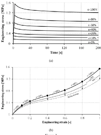
In addition to cyclic constant strain rate tensile tests, measurements were performed to examine the impact of strain rate on the stress-strain curve. During the test, specimens were loaded at a constant speed up to 100% strain level. Figure 2 shows the engineering stress-strain curves derived from the measured force- elongation curves by Eq. (1) and (2) at speeds of 1000, 500, 100 and 10 mm/min, corresponding to the strain rate of 0.27, 0.138, 0.027 and 0.00277 1/s, respectively.
There are differences in the values of the curves of identical features: tension at higher strain rate causes higher stress values at the same strain level. Despite the two orders of magnitude change in the strain rate, the stress difference at ε = 100 % strain is approximately 9%.
Figure 2
Engineering stress-strain curves of tensile tests at different strain rates
(a)
(b) Figure 3
(a) Engineering stress-time and (b) stress-strain curves of relaxation measurements at different strain levels up to t = 200 s
In order to study the time-dependent behaviour of isoprene rubber, stress relaxation tests were performed on specimens, similar to the ones applied for tensile tests. During the tests, after setting the 60 mm fixing length, the specimens were loaded to 5, 10, 20, 40, 60, 80 and 100% strain levels at a speed of v = 1000 mm/min (0.27 1/s strain rate), and stress relaxation was measured for t = 200 s.
Figure 3a shows the measured relaxation curves.
As can be seen, relaxation slowed down by t = 100 s at all strain levels. At t = 200 s, the differences between the maximum and relaxed values of the curves specified at each strain level are 28.68%, 26.39%, 24.61%, 23.46%, 22.99%, 22.77% and 22.64%, respectively.
Figure 3b shows the engineering stress-strain curves corresponding to the relaxation tests. The upload phases of relaxation tests can be considered as tensile tests of v = 1000 mm/min (similar to Figure 2). Furthermore, the figure specifies the relaxed stress values at each strain level after t = 200 s (see the broken line).
This broken curve can be considered as the relaxed tensile characteristic of the material.
As can be seen, the stress-strain curve of the 10 mm/min tensile test is very far from the relaxed state.
2 Analytical and Numerical Implementation of Finite Viscoelasticity
In engineering calculations, the behaviour of rubber is often considered to be independent of time, since calculations can be highly simplified this way. The theory of linear viscoelasticity can be applied if the material has considerable hysteresis at small strains. The theory of linear viscoelasticity is not appropriate for taking hyperelastic behaviour into consideration because, in this case, the stress-strain curve is not linear any longer. The theory of linear viscoelasticity was generalized by Simo in order to describe the mechanical behaviour of finite viscoelastic materials.
The II. Piola-Kirchoff stress (in the total Lagrange approach) by taking both strain and time dependence into account, is defined according to Eq. (3) [2]
n
1
i i
GL
GL,t) S ( ) T(t) (
S
(3) where S(εGL,t) is the II. Piola-Kirchoff stress depends on time and Green-Lagrange strain; S∞(εGL) is the II. Piola-Kirchoff stress in the relaxed state; while Ti(t) is an external variable specifying the time-dependence of the material with reference to term i of an n-term viscoelastic spring-dashpot model (see below). As can be observed, the first part of Eq. (3) describes the strain while the second part describes the time dependence. Dependence of the material model on strain will be taken into consideration in later chapters by the so-called Signiorini hyperelastic material model [1, 2].
c10 (I1( ) 3) c01 (I2( ) 3) c20 (I1( ) 3)2W (4)
where W(ε) is the specific strain energy density; c10, c01, and c20 are material constants; I1 and I2 are the first and second invariants of the Cauchy-Green strain tensor.
One of the most frequently applied spring-dashpot models demonstrating viscoelastic behaviour is the so-called Standard-Solid model, consisting of a linear spring parallel to the Maxwell element. The latter consists of a linear spring and a viscous element connected in series. A generalized Maxwell-model can be created by several Maxwell elements connected in parallel (see Figure 4), which -
similarly to the Standard-Solid model – can be used for modeling elastic and delayed elastic deformation components of rubbers. In applications where not only a qualitative but also a quantitative analysis is requested, a large number of Maxwell terms must be used (in many cases more than 20, see [5]).
Figure 4
n-term generalized Maxwell-model
The relaxation modulus of the generalized Maxwell-model can be specified according to Eq. (5)
i
n t
r 0 i
i 0
E (t) E E 1 e
(5)where Er(t) is the elastic modulus of the material at a given moment of relaxation;
E0 is the glassy modulus of the material; Ei and τi are the i-th modulus and relaxation time of the n-term generalized Maxwell-model. In practice, the i-th modulus of the generalized Maxwell-model is specified, instead of the Ei value, by an ei dimensionless energy parameter.
0 i
i E
e E and
1 0
1 E
e E
n
i i
. (6)Similarly to the theory of linear viscoelasticity, the external variable Ti(t) in Eq. (3) can be expressed in the form of a convolution integral as specified in Eq.
(7).
e S (t) e d) t (
T i
) T t t (
0 0 i
i
, (7)
where S0(t) is the time derivative of II. Piola-Kirchoff stress corresponding to the glassy state (see later).
Hereafter, the forms of Eq. (3) and (7) suitable for engineering calculations are specified with reference to a constant strain rate uniaxial tensile test. As a consequence of the convolution integral, calculations are performed incrementally
at Δt time intervals. The II. Piola-Kirchoff stress corresponding to the relaxed state is defined according to Eq. (8).
n
1 i GL i
GL 0
GL W ( ) 1 e
) ( S
, (8)
which, being expanded by the Signiorini material law can be seen in Eq. (9) and (10) for the relaxed and glassy states.
n
GL GL GL
10 20 1 01 2 i
i 1
S ( ) (c c ) (I ( ) c (I ( ) (1 e )
(9)0 GL GL GL
10 20 1 01 2
S ( )(c c ) (I ( ) c (I ( ) (10) By substituting the values of εGL in Eq. (9) and (10) by Eq. (11), the equations can be made dependent on t (v denotes the speed of tension).
2GL 1 m
2 1
where m
0 0
l v t
l l
(11)
The t dependent expression S0(t) can be used for specifying the external variable Ti(t) in the form of Eq. (12).
S (t) S (t t)
T(t t)e ) t (
Ti i i 0 0 i i , (12)
where
i t i 1 e
, (13)
t
i i
i
. (14)
The output parameters of the calculation are the Green-Lagrange strain and II. Piola-Kirchoff stress pairs. For the sake of comparability with the measurements, the stress and strain values were converted into engineering values by Eq. (15) and (16).
1 1 2 GL
m
(15)
m 1
PK
m
(16)
The calculation scheme can predict the mechanical behaviour of a rubber-like material by using any type of hyperelastic material law, if the Cauchy-Green strain tensor associated with the dominant type of loading (uniaxial tension, biaxial tension, simple shear and planar shear) is known and Eq. (4) can be expressed by its invariants. As seen, the above calculation schema works with the instantaneous values. Naturally a calculation scheme to be based on relaxation values can also be formulated [4, 7]. The resulted characteristics and values will be the same but the forms of equations will differ.
In the case of complex geometry or stress state, for example the finite element method (FEM) can be used to predict the material behaviour. [1, 2, 5]. In the MSC. Marc commercial FE software, the input parameters of a visco-hyperelastic analysis are constant material parameters defining the strain energy density corresponding to the glassy state (cij), as well as dimensionless energy parameters (ei) and relaxation times (τi) [2]. In order to take into consideration the incompressible nature of elastomers, special elements with Hermann formula can be applied.
3 Parameter Identification Based on Stress Relaxation Test
It is time-consuming and expensive to measure the time dependent behaviour of viscoelastic materials; therefore they are primarily used if the target is to describe the complex mechanical behaviour of the material in a broad frequency and temperature range, for which dynamic mechanical thermal analyzer (DMTA) measurements are widely applied. By shifting the isotherms measured by DMTA based on the time-temperature superposition, large generalized Maxwell-models (number of terms can reach 40) can be produced to cover frequency ranges which exceed even 20 orders of magnitude [6].
In the majority of problems occurring in engineering practice, viscoelastic models of a small number of terms can be used to describe time and frequency dependent behaviour with appropriate accuracy. These models represent the dynamic behaviour of the material in only a small frequency range; in the literature, it is recommended that the parameters be determined primarily by stress relaxation tests [2, 10].
In the event of stress relaxation, the rubber undergoes a completely elastic deformation as a consequence of a theoretically abrupt excitation of expansion.
Then the strain is kept constant and the rubber becomes delayed elastic with the stress decreasing from the initial maximum value, thus undergoing stress relaxation. In real tests, abrupt excitation of expansion is not possible: the loading phase is realized with a finite speed, so the relaxation partly takes place before the strain becomes constant. As a result, the maximum stress will not be identical with the maximum stress of the material with no relaxation in the loading phase.
The majority of FE softwares (Msc. Marc, Abaqus, Ansys) have built-in algorithms to fit the parameters of a characteristically 10-term generalized Maxwell-model to the relaxation test data. The curve fitting algorithm of Msc.
Marc performs this fitting to a shear modulus vs. time curve derived from the measurement. In this case, Eq. (5) contains the shear modulus of the material instead of its tensile modulus. In order to determine the shear modulus, the force- time curve yielded by the measurement must be converted into an engineering
stress-time curve by using Eq. (2) (see Figure 3a). The momentary or relaxation modulus of the material (Er) can be calculated by dividing the measured engineering stress values by the strain ε0 applied in the relaxation measurements.
The shear modulus can be calculated on the basis of the relaxation modulus curve by
3 ) 1 ( 2
E
G E
(17) where ν is the Poisson ratio of the material (in the case of incompressibility ν=0.5). In the course of fitting, the value of the glassy (or instantaneous) shear modulus G0 is also produced. Obviously, this is not identical with the real glassy modulus of the material because the loading phase was realized with a finite strain rate in the stress relaxation measurement. The traditional approach presented so far is only suitable for producing the parameters of a generalized Maxwell-model corresponding to small strain viscoelasticity, due to the fact that the dependence of G0 on strain is not taken into account. In order to introduce it, [2] proposes to substitute the value of E0 by a two parameter Mooney-Rivlin hyperelastic material law. The parameters can be estimated by using Eq. (18) and (19).
0 10 01
E 6 c c (18)
01 10
c 1
c 4 (19)
In the manner described, the parameters of viscoelastic model were produced on the basis of stress relaxation measured at strain level of 5, 60 and 100% (see Figure 3a). The parameters are shown in Table 2.
Table 2
Parameters specified on the basis of stress relaxation Strain level [%]
5 60 100
e1 [-] 0.0625 0.122 0.1176 e2 [-] 0.1289 0.0755 0.0870 e3 [-] 0.1076 0.0425 0.0309 τ1 [s] 0.1124 10.007 10.3299 τ2 [s] 11.0958 78.1938 83.7698 τ3 [s] 99.6630 123.54 137.777 E0 [MPa] 3.8804 1.36624 1.5461
Using these parameters, the FE method was applied for calculating the stress- strain and stress-time curves at a speed of 1000 mm/min. The material constants of the two parameter Mooney-Rivlin material law applied in the calculation were computed from the value of E0 specified in Table 2, using Eqs. (18) and (19). The FE model used is shown in Figure 5.
Figure 5
FE model and deformed shape of a standard specimen at 60 % strain
The model consists of 10400 linear hexahedron elements. The coefficient of friction between the rigid and meshed parts was μ = 2 in order to avoid slippage.
The rigid surfaces shown in Figure 5 approach each other according to the arrows indicated during the first 20 s of the calculation, in a way that the initial thickness (b0 = 10 mm) of the model is reduced to 6 mm. The next 300 s is a static phase of relaxation, followed by the motion of rigid surface in direction x, according to Figure 5. The speed of the motion was constant up to a prescribed strain value.
The stress relaxation occurs by keeping the rigid surfaces in a fixed position.
Similarly to the measurements, force and elongation values were collected from the calculation and converted into stress-strain and stress-time curves. Figures 6a and 6b show the results calculated for the phases of loading and relaxation, respectively. The calculations in Figure 6 are based on the viscoelastic parameters given in Table 2 and the Mooney-Rivlin parameters (c01, c10) computed from the glassy modulus (Eo) by Eqs. 18-19.
(a)
(b) Figure 6
Measured and calculated (a) stress-strain and (b) stress-time curves of the stress relaxation measurement
In order to quantify the differences between the curves, a so-called standard error is applied. In the case of an n number of x and y sampling values, the error can be calculated as
n
1 i
2 i i y) x n ( 1
. (20)
The behaviour measured is overestimated by the material law derived from stress relaxation at a strain of 5% – the standard error being 0.294 MPa – while it is significantly underestimated by those derived from relaxation at strain of 60% and 100 % with a standard error of 0.637 MPa and 0.560 MPa, respectively. One of the reasons for this is that at ε = 5%, the material had much less time to relax than at ε = 60 or 100%, so the E0 glassy modulus value determined here approximates the real value better. This difference is also affected by the ratio specified in Eq.
(19), which is a constant value independent of the material composition and test conditions. The characteristics of the curves calculated also considerably differ from the characteristics measured since the two parameter Mooney-Rivlin material law cannot provide a stress-strain curve having an inflexion point, which is typical with rubbers over a certain strain level. As indicated by the standard errors between the curves defined, the method proposed by [2] can be used for modeling the behaviour of rubbers primarily in the range of small strains, since in this case the stress relaxation occurring in the course of loading causes a smaller problem. Similarly, the difference between the behavior of the two-parameter Mooney-Rivlin material law and the real rubber is smaller at small strains than at large ones.
In order to partially solve the problems of the material laws derived from the relaxation test, the authors propose to apply a multi-parameter – e.g. the Signiorini hyperelastic – material model to be determined from the stress-strain curves of tensile tests. According to this, the free parameters of the hyperelastic model were
determined from tensile tests conducted at different speeds (see Figure 2) by using the curve fitting algorithm of MSC. Marc. Table 3 shows the fitted parameters and their ratios.
Table 3
Model parameters obtained from curve fitting
10minmm v
100minmm v
500minmm v
1000minmm v
c01[MPa] 1.2665 1.289 1.2835 1.3317
c10[MPa] -0.6382 -0.6697 -0.6905 -0.6774
c20[MPa] 0.1104 0.109 0.1099 0.1172
c01/ c10 [-] -1.9845 -1.9247 -1.8588 -1.9659 c10/ c20 [-] -5.7808 -6.1440 -6.2830 -5.7799
The ratios of parameters derived from separate tensile tests indicate small standard deviation; therefore, as a good approximation, they can be considered as identical regardless of the strain rate. Hereafter, the ratios of the 1000 mm/min tensile test will be used in the calculations.
As a first step, the parameters of the hyperelastic material model were recalculated by using the parameter ratios (see last column in Table 3) and the glassy modulus (E0 = 3.88 MPa from Table 2.) determined. To do this Eq. (4) was differentiated twice with respect to ε, yielding the E(ε) function. Substituting the value ε = 0 will produce the expression to describe the connection of E0 and the constant material parameters as shown in Eq. (21).
) c c ( 6
E0 10 01 (21)
(a)
(b) Figure 7
Comparison of measured and calculated (a) stress-strain and (b) stress-time curves As can be seen, Eq. (21) corresponds to Eq. (18) proposed by [2] for the two- parameter Mooney-Rivlin material law. Based on the parameter ratios and Eq.
(21), the recalculated material parameter values are c01 = 1.3163 MPa, c10 = 0.6696 MPa, and c20 = 0.1158 MPa, respectively. Figure 7a shows the measured and calculated (by using the recalculated parameters) loading phases of relaxation tests at ε = 100%.
As can be observed, the material law produced is capable of approximating the values measured much better than the calculation method proposed by [2]. In this case, the standard error of the loading phase is 0.0629 MPa, which is on an order of magnitude smaller than the former value. Figure 7b shows the measured and calculated relaxation phases of the relaxation test at 5%, 60% and 100% strain.
In all the cases, the calculations underestimate the measurements, which is a consequence of the lower glassy modulus (E0) value resulting from the relaxation test. The glassy modulus coming from stress relaxation measurement is smaller to the real value due to the stress relaxation during the loading phase. In the case of relaxation, the standard error between the calculation and the measurement is 0.01945 MPa, 0.0466 MPa, and 0.07519 MPa, respectively.
4 Parameter Identification from Simple Tensile Tests
The previous chapter showed the possibility of producing the parameters of a material law representing real mechanical behaviour through a stress relaxation test of small strain performed at the highest strain rate possible. However, the parameters can be obtained without a relaxation test, simply from two tensile tests of different speeds [11]. An advantage of this method is that the required material parameters, which are able to describe the mechanical behavior of the material in
a limited frequency and time range important in practice, can be produced with a minimum amount of tests.
The method is based on the recognition that the tensile tests with different strain rates result in different stress values at the same level of strain due to stress relaxation (Figure 2). From these differences the parameters of the spring-dashpot model (e.g. generalized Maxwell-model) can be identified. Figure 8 shows the block diagram of the method.
As seen, we need to calculate the first partial derivatives of the stress-strain curves of tensile tests measured at two different strain rates. This yields the elastic modulus-strain curves (EI(ε) and EII(ε)). Then the ratio of EI(ε) and EII(ε) values is calculated at different strains (Em(ε)). As a next step, the expression derived from Eq. (5) for the generalized Maxwell-model (Emfitted(ε)) is fitted to the Em(ε) values obtained by substituting the time parameter t with an expression including the length of the specimen, the tension speed and the strain (similarly to Eq. (11)).
The fitting itself can be performed with the method of least squares for models with a smaller number of terms or by genetic algorithm in the case of a higher number of terms. It is also possible to apply one of the increasingly-used optimization methods, e.g. the differential evolution (DE) algorithm detailed in [12].
The parameters of a 3-term generalized Maxwell-model were determined by the built in genetic algorithm of Matlab [13], using the 1000 mm/min and 10 mm/min measurement results of isoprene rubber. Table 4 shows the identified parameters.
Table 4 Identified parameters
ei [-] τi [s]
term 1 0.0756 0.101 term 2 0.0615 8.120 term 3 0.2039 91.891
Based on the analysis of the fitted parameters, it can be stated that the relaxation times correspond, with good approximation, to the relaxation times specified on the basis of the stress relaxation test at ε = 5%, but the sum of dimensionless energy parameters is Σei = 0.299 according to the relaxation measurement, while Σei = 0.341 on the basis of tensile tests.
If the viscoelastic parameters are known, then the glassy modulus can be determined from the equations presented in Figure 8. Contrary to the linear viscoelastic materials, where the glassy modulus has no strain dependency in the case of large strain viscoelasticity, the glassy modulus depends on the strain.
Figure 9 shows the glassy modulus determined from the 1000 mm/min uniaxial tensile test in function of strain.
Figure 8
Block diagram of the tensile test based parameter identification method
Figure 9
Glassy modulus identified by curve fitting in function of strain
The glassy modulus curve depicted is not linear and is not defined at ε = 0. Its value for the smallest ε is 4.27 MPa, which can be considered as the E0 glassy modulus of the material. The identified glassy modulus exceeds the 3.88 MPa value of the glassy modulus determined from the stress relaxation test at ε = 5%
strain. The glassy modulus (E0) and the parameter ratios in Table 3 can be used to determine the parameters of the Signiorini material law (c01 = 1.43798 MPa, c10 = -0.73146 MPa, and c20 = 0.12655 MPa).
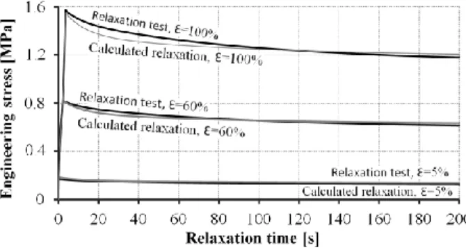
Figure 10 shows the measured and calculated characteristics of the relaxation tests measured at 5%, 60% and 100% strain, using the hyperelastic and viscoelastic parameters identified.
Figure 10
Comparison of simulation and measurement
As can be seen, the simulation differs slightly from measurement. After the nearly identical stress maximum, the calculated relaxation curve does not proceed parallel with the measured one, but intersects it at t = 120 s. The relative error between the measurement and the calculation is 0.01001 MPa, 0.0164 MPa and 0.03655 MPa, respectively.
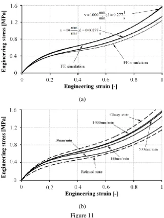
Figure 11a shows the measured and calculated tensile tests at 1000 mm/min and 10 mm/min tensile speed. At 10 mm/min the agreement is less good but the accuracy is still acceptable. The standard error of the simulation at higher speed is 0.008442 MPa, and that of the simulation at lower speed is 0.05626 MPa compared to the measurements.
The engineering stress-strain curves of the tensile tests were determined by analytical calculations as well, as shown in Figure 11b. The figure also shows the states corresponding to the glassy and relaxed state. The relaxed state shown in Figure 11b is lower than the one identified by measurement (Figure 3b). This is partly due to the fact that stress relaxation tests lasted for 200 s, which does not ensure that the final relaxed state is identified.
(a)
(b) Figure 11
(a) Calculated tensile tests of various speeds; (b) comparison of the engineering stress-strain curves of tensile tests with the calculated characteristics
Figure 12a shows the stress-strain curve of the measurement at 1000 mm/min, and Figure 12b shows that of the measurement at 10 mm/min, together with the results of the FE calculation using the material law set up on the basis of tensile tests and those of analytical calculations.
(a)
(b) Figure 12
Engineering stress-strain curves of the measurements, FE and analytical calculations at (a) 1000 mm/min and (b) 10 mm/min
As can be observed, the calculations at the higher speed approximate the results measured perfectly; the standard error of the FE calculation is 0.008442 MPa, while the error of the analytical calculation is 0.008398 MPa. As compared to the 10 mm/min measurement, the error of the FE calculation is 0.05626 MPa, while the error of the analytic calculation is 0.0672 MPa. The slight difference between the analytical and the FE calculations presumably follows from the discretization applied in the numerical adaptation of the equations presented in Chapter 2.
Conclusions
In the present paper, a new parameter identification method has been presented.
The proposed method enables the parameters of large strain generalized Maxwell- model to be determined on the basis of constant strain rate tensile tests. The application of the method has been presented for a specimen made of isoprene rubber. It has been proved that the method is able to identify large strain viscoelastic parameters of Maxwell-model with reasonable accuracy. In the event that one has only a standard tensile tester for material characterization, the proposed method is especially useful.
It will be shown in another paper that the proposed method can be used not only in the case of uniaxial tension, but also in the case of biaxial tension, simple shear, and planar shear.
Acknowledgements
This work is connected to the scientific program of the " Development of quality- oriented and harmonized R+D+I strategy and functional model at BME" project.
This project is supported by the New Széchenyi Plan (Project ID: TÁMOP- 4.2.1/B-09/1/KMR-2010-0002).
References
[1] S. Sharma, Critical Comparison of Popular Hyperelastic Material Models in Design of Anti-Vibration Mounts for Automotive Industry through FEA, Constitutive Models for Rubber III, 2003, ISBN 9058095665
[2] MSC. Marc. Volume A, Theory and User Information, Version 2007R1 [3] J. G. Barruetabeña, F. Cortés, J. M. Abete, P. Fernández, M. J. Lamela, A.
Fernández-Canteli, Experimental Characterization and Modelization of the Relaxation and Complex Moduli of a Flexible Adhesive, Materials and Design, 32(2011) pp. 2783-2796
[4] I. Németh, G. Schleinzer, R. Ogden, G. A. Holzapfel, On the Modeling of Amplitude and Frequency-Dependent Properties in Rubberlike Solids, Const. Models for Rubbers IV, Leiden, (2005) pp. 285-298
[5] L. Pálfi, T. Goda, K. Váradi, Numerical Modeling of Hysteretic Friction in Ball on Plate Configuration, eXPRESS Polymer Letters, Vol. 3, 11(2009) pp. 713-723
[6] D. Felhős, D. Xu, A. K. Schlarb, K. Váradi, T. Goda, Viscoelastic Characterization of an EPDM Rubber and Finite Element Simulation of its Dry Rolling Friction, eXPress Polymer Letters, Vol. 2, 3(2008) pp. 157- 164
[7] B. Marvalova, Identification of Viscoelastic Model of Filled Rubber and Numerical Simulation of Its Time Dependent Response, Vibration Problems, 126(2009) pp. 273-279
[8] A. F. M. S. Amin, A. Lion, S. Sekita, Y. Okui, Nonlinear Dependence of Viscosity in Modeling the Rate-Dependent Response of Natural and High Damping Rubbers in Compression and Shear: Experimental Identification and Numerical Verification, International Journal of Plasticity, 22(2006) pp. 1610-1657
[9] H. W. Müller, Experimental Identification of Viscoelastic Properties of Rubber Compounds by Means of Torsional Rheometry, Meccanica, 43(2008) pp. 327-337
[10] M. Herdy, Introductory Theory Manual ViscoData and ViscoShift, IBH- Ingenierbüro, 2003
[11] G. Bódai, T. Goda, Parameter Identification Methods for Generalized Maxwell-Models: Engineering Approach for Small-Strain Viscoelasticity, Materials Science Forum, 659(2010) pp. 379-384
[12] M. Ali, M. Pant, A. Abraham, Simplex Differential Evolution, Acta Polytechnica Hungarica, 6(2009) pp. 95-115
[13] Matlab, Version 7, The Language of Technical Computing, Genetic Algorithm and Direct Search Toolbox for Use with MATLAB User’s Guide, The Mathworks Inc, Natick, USA, 2004
![Table 4 Identified parameters e i [-] τ i [s] term 1 0.0756 0.101 term 2 0.0615 8.120 term 3 0.2039 91.891](https://thumb-eu.123doks.com/thumbv2/9dokorg/1233682.94775/15.748.268.482.605.687/table-identified-parameters-e-τ-term-term-term.webp)