Solving computational problems in real algebra/geometry

(1)

What does Mathematical Notation actually mean, and how can computers process it? ^∗

James H. Davenport

University of Bath (U.K.) J.H.Davenport@bath.ac.uk

Submitted September 14, 2014 — Accepted November 14, 2014

Abstract

Mathematical Notation is generally though of as universal and constant.

This is not as true as the layman thinks, and Notation is in fact an evolving, subject-specific, collection of sub-notations, where the same symbol can mean different things in different parts of the same sentence. This paper surveys the various ways computers process, and help humans to process, the varieties of notation.

Keywords:Mathematical Notation, MathML, OpenMath MSC:00A35, 68A30, 68C20

1. Notation: the perception and the reality

The outsiders’ perception of mathematical notation is that it is unambiguous, unchanging, precise, and world-wide (or more so¹). One need merely Google for the phrase “mathematically precise” to see many instances of this view. And indeed there is a lot of truth in this belief: the author has seen mathematicians be unable to speak to each other, having no human language in common, but be able to communicate by writing mathematics.

This is not just a popular belief: the computing discipline of “Formal Methods”, which employs tens of thousands of people in industry, as well as many academics,

∗Thanks to many people: typesetters, editors, OpenMath and MathML colleagues, TEXnicians.

1Witness various science-fiction stories where, e.g., Pythagoras’ Theorem is used as a demon- stration of intelligence.

http://ami.ektf.hu

47

(2)

Idea Anglo-Saxon French German half-open interval (0,1] ]0,1] varies single-valued function arctan Arctan arctan multi-valued function Arctan arctan Arctan

{0,1,2, . . .} N N N∪ {0}

{1,2,3, . . .} N\ {0} N\ {0} N Table 1: Cultural Notation Differences

tries to reduce computer programming to mathematics/logic, and has substantial success in doing so.

However, mathematical notation is certainly not unchanging. Few except the scholars of the history of notation would recognise in

1cu.m.6ce.p.11co.equale6nⁱ [2, attributed to [17]] the modernx³−6x²+ 11x= 6.

The + sign is less than 500 years old [19] (this text also introduced−andq ).

The = sign is slightly younger [18].

Recorde [18] wrote 2a+b: 2(a+b) is later, but the parenthetic notation won because it is (much!²) easier for manual typesetting.

Calculus had from the origin, and still has, two very different notations for ordi- nary differentiation: x˙ versus ^dx_dt, which have given rise touxxt versus _∂^∂²³_x∂t^u . Relativity introduced the summation convention [7]: P3

i=1cixⁱis abbreviated as cixⁱ (butcµx^µ is short forP3

µ=0cµx^µ, i.e. the range of summation depends on the alphabet from which the index is drawn).

Mathematical notation is also not quite as international as the layman believes:

see Table 1. The examples there are drawn from relatively advanced mathematics, but the differences can be more basic – [13, p. 2] lists five different forms of writing 9,435,671 found in Houston schools. These issues can spread to the description of algorithms such as division, as in Figure 1. Indeed MathML [22] recognises 10 such formats, such as stackedleftlinetop: see http://www.w3.org/Math/

draft-spec/mathml.html#chapter3_presm.mlongdiv.ex.

Mathematical notation is also subject-specific: while the mathematician writes ifor√

−1, the electrical engineer writesj, reservingifor current. A more chaotic

2The author, in the 1960s, used to typeset mathematics using “cold lead” technology: 2(a+b) involved selecting six characters from the cases of symbols, while 2a+b would have involved cutting a raised piece of lead to form the overlineand two “sleepers” – unraised pieces of lead – to sit either side of it to ensure that the overline was over the right characters. Furthermore, any change in the paragraph which moved thea+bhorizontally would involve cutting new sleepers.

(3)

Figure 1: Division (from [13, p. 7])

example of notational clash between subjects can be seen in [5], where the alge- braist uses [. . .]to indicate a polynomial ring extension, and the biochemist uses [. . .] to indicate “concentration of”. Hence computations were being conducted in C[[P][S][E]]. The fact that “reaction scheme” notation uses + to indicate combi- nation of reagents rather than mathematical addition is a further complication for the reader.

The mathematician also knows (without, possibly, having articulated it) that notation is area-specific within mathematics. For example(2,4)might be, depending on the area, any of:

Set Theory The ordered pair “first 2, then 4”;

(Geometry) The pointx= 2,y= 4;

(Vectors) The 2-vector of 2 and 4;

Calculus Open interval from 2 to 4;

Group Theory The transposition that swaps 2 and 4;

Number Theory The greatest common divisor of 2 and 4;

(4)

In general, these expressions, whilst written identically, are spoken differently by the mathematician: the written text “we draw a line from(2,4)to(3,5)” is spoken

“we draw a line from the point(2,4)to the point(3,5)”. This can apply even within a given sentence³: every group theorist would read

SinceHi≤Gfori≤n (1.1)

as “SinceH subiis a subgroup ofGforiless than or equal ton” without, probably, even noticing that the two instances of ≤ had been pronounced very differently.

This issue is a major challenge for mathematics “text-to-speech” renderers.

2. Imperfections in notation

Mathematical notation has evolved over the centuries, and some innovations were, with hindsight, less than ideal.

2.1. “Landau” Notation

This notation, apparently actually due to Bachmann [3], has two components. The first is not controversial: we useO(f(n))to denote those functions that “grow no faster thanf(n)” – formally (though rarely stated as such)

O(f(n)) ={g(n)|∃N, A:∀n > N |g(n)|< Af(n)}, (2.1) and similarly with o, Ω, ω and Θ. The second component of this notation is the use of “=” with this, as in log₂n = O(logn). This is not the traditional use of the=sign, as the relation is not symmetric: we can’t writeO(logn) = log₂n, for example, and while we might stretch the notation toO(n²) =O(n³), it is certainly not the case that O(n³) = O(n²). Again, the spoken language gives a clue: the (English-speaking) mathematician would say “is” not “equals”.

If we were honest with (2.1), we would writeO(logn)∈log₂n, but to the best of the author’s knowledge, [12] is the only textbook to be consistently honest in this area using ∈, though [9] does refer to O(f) as a set, and is careful to use neither = nor ∈. Being honest with (2.1) has another advantage: we can write Θ(f(n)) =O(f(n))∩Ω(f(n)), as [9] does.

2.2. Iterated Functions

No-one could quarrel with any of the following:

sin(x²) squarex, then applysin

(sinx)² apply sintox, then square the result sin(sin(x)) applysin tox, then applysinagain

3I owe this example to Ieuan Evans of Bath.

(5)

The problem comes withsin²x, which is generally used to mean(sinx)², whereas, if anything, it should mean sin(sin(x)), since this is the sense in which we write sin⁻¹(x)– apply the inverse operation ofsin, not1/sin(x). The author is not the first to object to this notation: “[This] is by far the most objectionable of any”

[2]. The author has not encountered a definitive explanation of the origin of this notation, which was clearly common by the time of Babbage, but his experience of manual printing leads him to believe that it was economy of printing:

sin²θ+φ

2 versus

sinθ+φ 2

2

obviates searching for the very large brackets, and building up an exponent to a non-standard height.

2.3. Continued Fractions

The “correct” notation for continued fractions, as in

π= 3 + 1

7 + ₁₅₊ ¹1 1+ 1

292+...

(2.2)

is nearly always reduced to

π= 3 + 1 7+

1 15+

1 1+

1

292+· · · , (2.3)

which is much easier for (manual) typesetting⁴, and uses less space – still a relevant consideration. Furthermore, if the individual terms of the continued fraction are complicated, as in

α=a0+ 1

a1+_a ¹

2+ ¹

a3+ 1 a4+...

,

the alternative notation is probably more readable, at least when the reader is used to it.

2.4. Conclusion

We actually see that the same printed notation can mean very different mathematical objects, and that the same mathematical object can be displayed in many different styles. This has led to a conceptual split between the computerisation of the presentation, how the mathematics looks, and the computerisation of the content (or semantics), i.e. what the mathematics means. This is formalised in the MathML standard, which has different chapters, and even different basic tokens, for the two approaches.

4As we (L^ATEX) have written it (2.2) uses three sizes of digits, while (2.3) only uses one. Most

“Hot metal” printers only had two available, so the result would not be as attractive as (2.2).

(6)

3. Computer Displays of Mathematics

Let us first look at how computers mediate the presentation of mathematical formulae.

3.1. Display of Mathematics

We can distinguish various (overlapping) periods in the computer display of mathematics.

1. Images – generally GIF or JPEG formats, though others have been used, and SVG has become more desirable [20]. The fundamental problem with an image is that it is precisely an image – all machine-processable information has been lost. In HTML, it is possible to include anALTernative representation, and this might be the L^ATEX source, which at least conveys some information to a text-to-speech renderer.

2. Computer processing – as photocomposition replaced “hot metal” technology in typesetting shops, so these photocomposers became computer-controlled.

Various programs, notably troff [16] and the associated mathematics pre- processoreqn[10], were developed to take advantage of this capability, and the author’s PhD thesis was ported as [6] to the IBM equivalent program – YFL [8].

3. A major breakthrough came with Knuth’s TEX [11]. One fundamental de- velopment here over its predecessors was the principle of boxes with width, height and depth. The requirement to know the explicit depth of a box is fundamental, as in (2.2). This has become the de facto gold standard for mathematical typesetting.

4. The original HTML did not support mathematics, much to its designer’s regret, and MathML–Presentation 1.0 [21] soon appeared to fill this gap.

However, the browsers of the period did not support the concept of ‘depth’ for boxes, and this can still be a problem today (Chrome’s support for MathML has been intermittent, largely for this reason). A further challenge with many browsers⁵ is the lack of fonts available.

5. MathJax [14] has emerged as a pragmatic solution to the vagaries of browsers, and is discussed further in [20].

3.2. Line Breaking

All systems the author knows of make a fundamental distinction between “in-line”

and “display” mathematics, and the user has to state which is required, e.g. $...$

versus$$...$$ in TEX. TEX and its derivatives provide so support for automatic

5And other software: PowerPoint has often given users problems here.

(7)

breaking of lines if a displayed formula overflows the line width, and not much support for in-line formulae⁶. In the author’s experience, a significant fraction of the effort in converting a paper from one format to another is in reflowing the equations, and maybe converting from display to in-line orvice versa.

However, the author of a web page has no control over the width within which it is displayed, and hence the browser must dosomething about linebreaking. This is also a problem for the various kinds of e-book readers, and partially accounts for the relative difficulty of handling mathematics, or technical text in general, on these devices. The MathML standard [23, §3.1.7] provides a suggested algorithm, but, as it says there:

This algorithm takes time proportional to the number of token elements times the number of lines.

This problem, with its blend of algorithmics and aesthetics, is at least as difficult as, but less-researched than, the problem of table layout, as discussed in [15]

3.3. MathML-Presentation

While it is possible to regard MathML-Presentation as “L^ATEX with pointy brackets”, this view in fact does it a disservice. While f(x), written asf(x) in TEX, could be written as

it would best be represented in MathML as

<mrow>

<mrow>

</mrow>

In this representation, the function application, and precisely what the argument is, are clearly apparent. This matters for speech rendering – “f of x”, as well as semantic analysis. However, it is still presentation, and cannot solve the sort of problem seen in (1.1).

6TEXnically speaking, the mathematics has been converted into a list of boxes by the time it is realised that line-breaking is needed, hence rules like “break at the outermost operator” no longer make sense.

(8)

4. Computer Representation of Mathematical Con- tent

Originally, there were two different approaches to the description of mathematical content: OpenMath and MathML-Content. We describe each, and then the convergence process.

4.1. OpenMath

The OpenMath movement grew out of the Computer Algebra community’s wish to move formulae between systems. An early document is [1], which emphasises the importance of extensibility. Indeed, OpenMath is not so much an encoding as a framework for encoding, and the Standard [4] does not of itself specify how to transmit anything more complicated than integers. In fact it defines only a few basic concepts, listed here as their XML encodings.

OMOBJ The basic constructor, whose argument is an OpenMath objects. This exists so that OpenMath can be embedded in other documents, as formulae are in text. It’s opposite isOMFOREIGN, indicating that we have some non-OpenMath constructs (such as Presentation MathML) embedded in an OpenMath object.

OMS This indicates an “OpenMath Symbol”, an object to which the OpenMath process assigns a definite meaning. The arguments are thenameof the symbol, e.g. sin, and the location of the “Content Dictionary” in which that definition can be found. This location can be either a simple name (transc1 would indicate the standard Content Dictionary for basic transcendental functions) or a complete URL.

OMA This indicates an “OpenMath Application”, where the first argument is to be considered an operator applied to the remaining arguments.

OMBIND This indicates an “OpenMath Binding”, where the first argument is some operator to bind the variables specified in the second argument in the use of the third argument. A typical first argument would be

<OMS name="forall" cd="quant1"/>to indicate∀.

OME This indicates an “OpenMath Error Object” (such as “divide by zero”): the first argument is the ‘name’ of the error, as anOMS, and the rest are additional arguments depending on the error.

OMATTR This indicates an “OpenMath Attribution”: the first argument has various attributes, such ascolorbeing red.

OMR This indicates an “OpenMath Reference” and allows us to build directed acyclic⁷ graphs, rather than just trees.

7There is an explicit ban on cycles in the OpenMath standard.

(9)

Basic objects are encoded by any ofOMV (variables), OMI (integers), OMB (byte arrays),OMSTR(Unicode strings) orOMF(IEEE floating-point numbers).

4.2. MathML-Content

This was introduced at the start of the MathML process, with a view to being

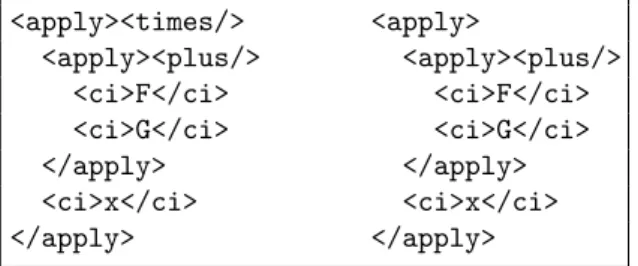
“an explicit encoding of the underlying mathematical meaning of an expression, rather than any particular rendering for the expression” [23]. Equally, as have we have seen, renderings can be ambiguous, and one aim of MathML-Content is to remove this ambiguity. Consider (F+G)x: this could be either multiplication or function application: see Figure 2. We note that there is no need for brackets, as

</apply> </apply>

</apply> </apply>

Figure 2: Alternative MathML-Content for(F+G)x

<apply>. . .</apply>groups, and the meaning is explicit: in the first we have an application of <times/>while in the second we are applyingF+G.

The original aim in MathML (version 1) was to handle “school” mathematics, otherwise “K–12”, or Kindergarten to 12th-grade. However, this became a moving target, as constructs like<div>were introduced.

4.3. Convergence

The reader will have noticed that there is a strong similarity between OpenMath and MathML-Content, with<apply>corresponding to<OMA>, and<ci>constructs corresponding to <OMV name= constructs. The difference is that <plus/> is part of the MathML specification, whereas<OMS name="plus" cd="arith1"/>is just a symbol in an OpenMath content dictionary. This difference is also the source of the greater expressivity of OpenMath: MathML needed to charge to accommodate

<div/>, whereas OpenMath just added theveccalc1content dictionary.

MathML version 2 therefore added the ability to use OpenMath symbols, thus buying into the expressivity of OpenMath. In MathML version 3, the authors went further, and defined MathML-Content in terms of OpenMath as follows.

[In §4.2] a core collection of elements comprising Strict Content Markup are described. Strict Content Markup is sufficient to encode general expression trees in a semantically rigorous way. It is in one-to-one

(10)

correspondence with OpenMath element set. OpenMath is a standard for representing formal mathematical objects and semantics through the use of extensible Content Dictionaries. [23, §4.1.1].

<plus/>is then defined to be a shorthand for<OMS name="plus" cd="arith1"/>, etc.

5. Conclusion

In terms of reproducing via computers the intricate two-dimensional layouts of mathematical notation, created (at considerable expense) by cold-metal printers, the TEX engine [11] has no equal. However, all it does is express how to lay out the symbols, and says nothing about their meaning. The invisible operator after) in the L^ATEX(F+G)xcould be either function application or multiplication.

Although it is possible to write MathML-presentation that conveys no more information than the L^ATEX, well-written MathML-presentation can convey far more, as the invisible operator should be either⁡or⁢.

However, presentation MathML can only go so far in encoding meaning, and is still unable to resolve the two uses of ≤ in (1.1) for example. For this, we need a representation of the semantics ,either OpenMath or MathML-Content.

Fortunately, the two have converged so much that they are essentially isomorphic structures, and we can look forward to greater convergence in the future.

References

[1] J.A. Abbott, A. Díaz, and R.S. Sutor. OpenMath: A Protocol for the Exchange of Mathematical Information. SIGSAM Bulletin 1, 30:21–24, 1996.

[2] C. Babbage. Article “Notation”. Edinburgh Encyclopaedia, 15:394–399, 1830.

[3] P. Bachmann. Die analytische Zahlentheorie. Teubner, 1894.

[4] S. Buswell, O. Caprotti, D.P. Carlisle, M.C. Dewar, M. Gaëtano, and M. Kohlhase.

The OpenMath Standard 2.0. http://www.openmath.org, 2004.

[5] J.P. Bennett, J.H. Davenport, M.C. Dewar, D.L. Fisher, M. Grinfeld, and H.M.

Sauro. Computer algebra approaches to enzyme kinetics. In Gérard Jacob and Françoise Lamnabhi-Lagarrigue, editors, Algebraic Computing in Control, volume 165 of Lecture Notes in Control and Information Sciences, pages 23–30. Springer Berlin Heidelberg, 1991.

[6] J.H. Davenport. On the Integration of Algebraic Functions, volume 102 ofSpringer Lecture Notes in Computer Science. Springer Berlin Heidelberg New York (Russian ed. MIR Moscow 1985), 1981.

[7] A. Einstein. Die Grundlage der allgemeinen Relativitaetstheorie (The Foundation of the General Theory of Relativity). Annalen der Physik Fourth Ser., 49:284–339, 1916.

(11)

[8] A.M. Gruhn. The Yorktown Formatting Language: User Guide. Technical Report RC 6994 IBM Research, 1979.

[9] M. Hetland.Python algorithms: Mastering Basic Algorithms in the Python Language (2nd ed.). Apress, 2014.

[10] B.W. Kernighan and L.L. Cherry. A System for Typesetting Mathematics. Comm.

ACM, 18:151–157, 1975.

[11] D.E. Knuth. The TEXbook: Computers and Typesetting Vol. A. Addison–Wesley, 1984.

[12] A. Levitin. Introduction to the design and analysis of algorithms. Pearson Addison–

Wesley, 2007.

[13] N.R. Lopez. Mathematical Notation Comparisons between U.S. and Latin Ameri- can Countries. https://sites.google.com/site/algorithmcollectionproject/

mathematical-notation-comparisons-between-u-s-and-latin-american- countries, 2008.

[14] MathJax Consortium. MathJax: Beautiful math in all browsers. http://www.

mathjax.org/, 2011.

[15] Kim Marriott, Peter Moulder, and Nathan Hurst. Html automatic table layout.

ACM Trans. Web, 7(1):4:1–4:27, March 2013.

[16] J.F. Ossanna. Nroff/Troff User’s Manual. Technical Report 54 Bell Labs, 1976.

[17] Luca Pacioli. Summa de arithmetica, geometria, proportioni et proportionalita.

Venice, 1494.

[18] R. Recorde. The Whetstone of Witte. J. Kyngstone, London, 1557.

[19] Stifelius [Michael Stifel]. Arithmetica Integra. Iohan Petreius, Norimberg, 1544.

[20] M. Schubotz and G. Wicke. Mathoid: Robust, Scalable, Fast and Accessible Math Rendering for Wikipedia. http://arxiv.org/abs/1404.6179, 2014.

[21] World-Wide Web Consortium. Mathematical Markup Language: First Public Draft.

http://www.w3.org/TR/WD-math-970515/, 1997.

[22] World-Wide Web Consortium. Mathematical Markup Language (MathML) Version 3.0: W3C Recommendation 21 October 2010. http://www.w3.org/TR/2010/REC- MathML3-20101021/, 2010.

[23] World-Wide Web Consortium. Mathematical Markup Language (MathML) Version 3.0: second edition. http://www.w3.org/TR/2014/REC-MathML3-20140410/, 2014.