ANALYTICAL AND FINITE ELEMENT SOLUTION OF A SIMPLY SUPPORTED PLATE SUBJECTED TO
HYDROSTATIC LOAD
Author: Dr. András Szekrényes
13.
ANALYTICAL AND FINITE ELEMENT SOLUTION OF A SIM- PLY SUPPORTED PLATE SUBJECTED TO HYDROSTATIC LOAD
Calculate the deflection surface, the distribution of bending and twisting moments and stresses in the plate under hydrostatic load shown in Fig.13.1 by
a. analytical method utilizing the basic equations of thin plates, b. finite element method using the code ANSYS 12,
and finally, make a comparison of the results obtained by the two different calculations!
The material of the plate is linear elastic, homogeneous and isotropic.
Fig.13.1. Simply supported plate subjected to hydrostatic load.
Given:
E = 200 GPa, ν = 0,3, a = 500 mm, b = 350 mm, t = 2 mm, p0 = 10 kN/m2. 13.1 Analytical solution
In section 12 we have already derived the governing partial differential equation for the deflection surface w(x,y) of bent plates [1] (see Eq.(12.31)):
1 1 4 4 2 2 4 4
4 ( , )
2 I E
y x p y
w y
x w x
w =
∂ +∂
∂ + ∂
∂
∂ , (13.1)
where I1 = t3/12, E1 = (E/(1-ν2), p(x,y) is the function of the load distributed on the plate surface. For simply supported plates the displacement and bending moment are zero on the corresponding boundaries, i.e. the boundary conditions are:
0 ) , 0 ( y =
w ,w(a,y)=0,w(x,0)=0,w(x,b)=0, (13.2) 0
) , 0 ( y =
Mx ,Mx(a,y)=0,My(x,0)=0,My(x,b)=0
Based on Eq.(12.7) (see section 12) the relationship between the bending moments and the deflection function is:
)
( , ,
1
1 xx yy
x I E w w
M =− +ν ⋅ ,My =−I1E1(w,yy +ν ⋅w,xx), (13.3) xy
xy I E w
M =− 1 1(1−ν) , ,
viz., the boundary conditions with respect to the bending moments can be reformulated using the deflection function. The boundary conditions can be satisfied if we develop the solution using a double sine series in terms of both the x and y variables. The solution func- tion is [1,2]:
∑∑
∞=
∞
=
⋅
=
1 1
) sin(
) sin(
) , (
n m
mn x y
W y
x
w α β , (13.4)
where Wmn, α and β are the coefficients of the solution, and:
a mπ α = ,
b nπ
β = . (13.5)
The load function is provided in the form of a similar series:
∑∑
∞=
∞
=
⋅
=
1 1
) sin(
) sin(
) , (
n m
mn x y
Q y
x
p α β . (13.6)
where Qmn is the coefficient of the approximate function of the load. To obtain the solution we utilize the followings [1,2]:
=
= ≠
∫
nby ⋅ lby b nn llb
if , 2 /
if , ) 0 sin(
) sin(
0
π
π . (13.7)
We multiply p(x,y) with sin(lπy/b) and then we integrate it from 0 to b with respect to y:
) 2 sin(
) sin(
) , (
0 1 a
x Q m
dy b b
y y l
x p
m ml
b π
∑
π∫
∞=
⋅
=
⋅ (13.8)
Let us multiply both sides with sin(kπx/a) and integrate it with respect to x from 0 to a:
kl a b
abQ a dydx
x k b
y y l
x
p( , ) sin( ) sin( ) 4
0 0
=
⋅
∫ ∫
⋅ π π , (13.9)Since we can exchange the indices we obtain:
∫∫
⋅ ⋅=
a b
mn dydx
b y n a
x y m
x ab p
Q
0 0
) sin(
) sin(
) ,
4 ( π π
. (13.10) Next, we calculate the derivatives of the solution function:
∑∑
∞=
∞
=
⋅
−
∂ =
∂
1 1
2 2
2
) sin(
) sin(
n m
mn x y
x W
w α α β , (13.11)
∑∑
∞=
∞
=
⋅
−
∂ =
∂
1 1
2 2
2
) sin(
) sin(
n m
mn x y
y W
w β α β ,
∑∑
∞=
∞
=
⋅
∂ =
∂
∂
1 1
2
) cos(
) cos(
n m
mn x y
y W x
w αβ α β ,
∑∑
∞=
∞
=
⋅
∂ =
∂
1 1
4 4
4
) sin(
) sin(
n m
mn x y
x W
w α α β ,
∑∑
∞=
∞
=
⋅
∂ =
∂
1 1
4 4
4
) sin(
) sin(
n m
mn x y
y W
w β α β ,
∑∑
∞=
∞
=
⋅
∂ =
∂
∂
1 1
2 2 2
2 4
) sin(
) sin(
n m
mn x y
y W x
w α β α β .
{ }
∑∑
∞=
∞
=
=
⋅ +
+ +
−
1 1
4 2 2 4 1
1 ( 2 ) sin( ) sin( ) 0
n m
mn
mnI E Q x y
W α α β β α β ,
(13.12)
and the equation above must be satisfied independently of the location, i.e. the nontrivial solution is:
1 1 2 2
2 )
( I E
Wmn α +β = Qmn , (13.13)
and:
2 2 2
4 1 1 2 2 2 1
1 ( ) I E ((m/a) (n/b) )
Q E
I
Wmn Qmn mn
= +
= +
π β
α . (13.14)
Taking it back into the solution function we obtain the following:
∑∑
∞=
∞
=
+ ⋅
=
1 1
2 2 2 1 1
) sin(
) ) sin(
) ( , (
n m
mn x y
E I y Q
x
w α β
β
α . (13.15)
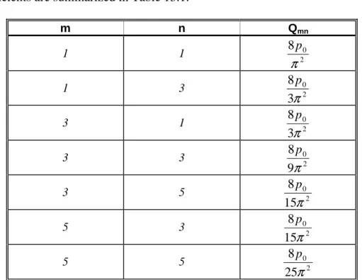
Accordingly, the solution function is obtained in terms of the coefficients of the load func- tion. For the case of hydrostatic load the coefficients can be produced relatively easy based on Eq.(13.7) since p(x,y) = p0⋅x/a [1,2]:
) 8 cos(
) sin(
) 4 sin(
2 0 0 0
0 π
π π
π m
mn dydx p
a x m b
y n a p x Q ab
a b
mn =
∫ ∫
⋅ ⋅ =− , m, n = 1, 3, 5..∞.(13.16) The coefficients are summarized in Table 13.1.
m n Qmn
1 1 8 20
π p
1 3 02
3 8 π
p
3 1 02
3 8 π
p
3 3 20
9 8 π
p
3 5 02
15 8
π p
5 3 02
15 8
π p
5 5 02
25 8
π p
Table 13.1. Coefficients of the load function of a simply supported plate.
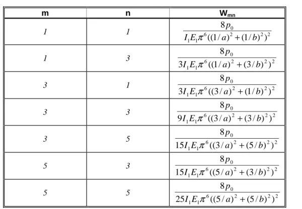
Calculate now the Wmn coefficients of the solution functions. The results are summarized in Table 13.2.
m n Wmn
1 1 6 2 2 2
1 1
0
) ) / 1 ( ) / 1 ((
8
b a
E I
p π +
1 3 6 2 2 2
1 1
0
) ) / 3 ( ) / 1 ((
3
8
b a
E I
p π +
3 1 6 2 2 2
1 1
0
) ) / 1 ( ) / 3 ((
3
8
b a
E I
p π +
3 3 6 2 2 2
1 1
0
) ) / 3 ( ) / 3 ((
9
8
b a
E I
p π +
3 5 6 2 2 2
1 1
0
) ) / 5 ( ) / 3 ((
15
8
b a
E I
p π +
5 3 6 2 2 2
1 1
0
) ) / 3 ( ) / 5 ((
15
8
b a
E I
p π +
5 5 6 2 2 2
1 1
0
) ) / 5 ( ) / 5 ((
25
8
b a
E I
p π +
Table 13.2. Coefficients of the solution function of a simply supported plate.
It can be seen that we calculated only seven coefficients, with that the deflection function becomes:
5 ).
sin(
5 ) sin(
3 ) sin(
5 ) sin(
5 ) sin(
3 ) sin(
3 ) sin(
3 ) sin(
) sin(
3 ) sin(
3 ) sin(
) sin(
) sin(
) sin(
) sin(
) sin(
) , (
55 53
35 33
31
13 11
1 1
b y a
W x b
y a
W x
b y a
W x b
y a
W x b
y a
W x
b y a
W x b
y a
W x y x
W y
x w
n m
mn
π π
π π
π π
π π
π π
π π
π β π
α
⋅ +
⋅ +
+
⋅ +
⋅ +
⋅ +
+
⋅ +
⋅
=
⋅
=
∑∑
∞=
∞
=
(13.17)
The displacement in direction z in the midpoint of the plate was calculated by increasing the number of the considered coefficients. In the first case we considered only W11, in the second case we included W11 and W13 too, etc. The results are summarized in Table 13.3 where it is shown that the displacement rapidly converges to a given value.
number of Wmn coeffi-
cients [pcs]
1 2 3 4 5 6 7
w(a/2,b/2)
[mm] -3.8388 -3.8072 -3.7102 -3.7154 -3.7148 3.7135 3.7138
Table 13.3. The convergence of the midpoint displacement of the plate increasing the number of coefficients.
Fig.13.2. Deflection function of a simply supported plate subjected to hydrostatic load, the unit is in [m].
The deflection function is plotted in Fig.13.2, where all of the seven coefficients were taken into account. The maximum displacement takes place in the midpoint of the plate.
The bending moments can be obtained using Eq.(13.3):
∑∑
∞=
∞
=
⋅ +
=
⋅ +
−
=
1 1
2 2 1
1 , ,
1
1 ( ) ( )sin( ) sin( )
n m
mn yy
xx
x I E w w I E W x y
M ν α νβ α β ,
(13.18)
∑∑
∞=
∞
=
⋅ +
=
⋅ +
−
=
1 1
2 2 1
1 , ,
1
1 ( ) ( )sin( ) sin( )
n m
mn xx
yy
y I E w w I E W x y
M ν να β α β ,
∑∑
∞=
∞
=
⋅
−
=
−
−
=
1 1
1 1 , 1
1 (1 ) (1 ) cos( ) cos( )
n m
mn xy
xy I E w I E W x y
M ν ν αβ α β ,
where Mx is the bending moment along x, My is the bending moment along y, Mxy is the twisting moment, respectively. The functions of the moments are shown by Figs.13.3-13.5.
Fig.13.3. Distribution of the Mx bending moment in a simply supported plate subjected to hydro- static load, the unit is in [Nm/m].
Fig.13.4. Distribution of the My bending moment in a simply supported plate subjected to hydro- static load, the unit is in [Nm/m].
Fig.13.5. Distribution of the Mxy twisting moment in a simply supported plate subjected to hydro- static load, the unit is in [Nm/m].
The shear forces can be calculated based on the equilibrium equations given by Eqs.(13.19) and (13.20) of section 14:
x x
yy xx x xy
x I E w w I E w
y M x
Q M =− 1 1( , + , ), =− 1 1(∆ ),
∂
−∂
∂
= ∂ , (13.19)
y y
yy xx y
yx
y I E w w I E w
y M x
Q M =− 1 1( , + , ), =− 1 1(∆ ),
∂ +∂
∂
= ∂ .
The function plots of the shear forces are given in Figs.13.6 and 13.7.
Fig.13.6. Distribution of the Qx shear force in a simply supported plate subjected to hydrostatic load, the unit is in [N/m].
Fig.13.7. Distribution of the Qy shear force in a simply supported plate subjected to hydrostatic load, the unit is in [N/m].
The stresses are obtained by using the following formulae [1,2]:
I z Mx
x 1
σ = , z
I My
y 1
σ = , z
I Mxy
xy 1
τ = , (13.20)
where I1 = t3/12 is the second order moment of inertia of the plate. Due to the fact that the stresses are proportional to the moments at a given z coordinate, the stress distributions are not given here. The normal stresses at the point with coordinate z = -t/2 in the midpoint of the plate are:
MPa 10 , 2 44 ) 2 / , 2 / (
1
−
=
= t
I b a Mx
σx , (13.21)
MPa 36 , 2 69 ) 2 / , 2 / (
1
−
=
= t
I b a My
σy .
The maximum value of the shear stress takes place at the point where x = a and y = b, i.e.:
MPa 38 , 2 53 ) , (
1
=
= t
I b a Mxy
τy . (13.22)
13.2 Finite element solution
Solve the plate problem shown in Fig.13.1 by the finite element method too! Prepare the finite element model of the plate shown in Fig.13.1 and calculate the nodal displacements and stresses! Plot the distribution of the bending and twisting moments, normal and shear stresses on the surface of the plate!
The finite element solution is presented by using the code ANSYS 12. The actual com- mands are available in the left hand side and upper vertical menus [3]. The distances are defined in [m], the force is given in [N].
Printing the problem title on the screen
File menu / Change Title / Title: “Simply supported plate subjected to hydrostatic load”
- refresh the screen by the mouse roller Analysis type definition
PREFERENCES – STRUCTURAL
Element type definition – 4 node shell element (SHELL63)
PREPROCESSOR / ELEMENT TYPES / ADD/EDIT/DELETE / ADD / SOLID / ELAS- TIC 4NODE 63 / OK /
PREPROCESSOR / REAL CONSTANTS / ADD/EDIT/DELETE / ADD / OK / Shell thickness at node I TH(I) = 0.002 / OK - definition of the thickness Material properties definition
PREPROCESSOR / MATERIAL PROPS / MATERIAL MODELS / STRUCTURAL / LINEAR / ELASTIC / ISOTROPIC / EX = 200e9, PRXY = 0.3 / OK Exit: Material menu / Exit
Geometry preparation
PREPROCESSOR / MODELING / CREATE / AREAS / RECTANGLES / BY 2 COR- NERS / WPX = 0, WPY = 0, WIDTH = 0.5, HEIGHT = 0.35
- definition of the coordinates in the opening window
The surface of the plate is shown by Fig.13.8. Click the 9th icon on the right entitled „Fit View”, it fits the screen to the actual object size. Clicking the 1st icon on the right, entitled
„Isometric View” we can view the model in 3D.
Fig.13.8. Surface of a simply supported plate.
Meshing
Element number definition along the boundary lines
PREPROCESSOR / MESHING / SIZE CNTRLS / MANUALSIZE / LINES / PICKED LINES / PICK / NO. OF ELEMENT DIVISIONS = typing in the proper number, repetition of the command
- along the edges parallel to axis x we define 50 elements - along the edges parallel to axis y we define 35 elements
PREPROCESSOR / MESHING / MESH / AREAS / MAPPED / 3 OR 4 SIDED / PICK ALL
Plot menu / Multi-Plots - display the elements and nodes
The finite element mesh of the plate is demonstrated in Fig.13.9.
Fig.13.9. Finite element mesh of a simply supported plate.
Kinematic constraints definition
PREPROCESSOR / LOADS / DEFINE LOADS / APPLY / STUCTURAL / DIS- PLACEMENT / ON LINES
- selection of the four boundary curves / OK / UZ / APPLY
- selection of the boundary curve at x = 0 / OK / UX / APPLY - selection of the boundary curve at y = 0 / OK / UY / OK
The constraints are represented by small arrows acting in the proper directions, as it is shown by Fig.13.10.
Fig.13.10. Kinematic boundary conditions of a simply supported plate.
Loading definition, linearly distributed load
The slope of the distributed load function is p0/a = 10000/0,5 = 20000 N/m3
PREPROCESSOR / LOADS / DEFINE LOADS / SETTINGS / FOR SURFACE LD / GRADIENT / SLOPE = - 20000 – value of the slope
SLDIR = X – the direction of the linear change
SLZER = 0 – coordinate location where slope contribution is zero
PREPROCESSOR / LOADS / DEFINE LOADS / APPLY / STUCTURAL / PRESSURE / ON AREAS / VALUE Load PRES Value = 0 (explanation: the slope and the “SLZER”
were defined before)
Display the arrows of the distributed load
PlotCtrls menu / Symbols / Surface Load Symbols: “Pressures”
Show pres and convect as: „Arrows”
Solution
SOLUTION / SOLVE / CURRENT LS
„SOLUTION IS DONE!”
Plotting and listing of the results
GENERAL POSTPROC / PLOT RESULTS / DEFORMED SHAPE / select Def + undef edge / OK
PlotCtrls menu / Animate / Deformed Shape - animation
NODAL SOLUTION: nodal displacements
DOF SOLUTION: UX, UY, USUM displacements with color scale
STRESS: normal and shear stresses, principal stresses, equivalent stresses
ELASTIC STRAIN: strains and shear strains, principal strains equivalent strains
Fig.13.11. Transverse displacement (z) of a plate under hydrostatic load in [m].
Transverse displacement of the points of the plate is shown in Fig.13.11, where it is shown that the maximum displacement takes place in the midpoint of the plate, its value is: 3,83 mm.
GENERAL POSTPROC / PLOT RESULTS / CONTOUR PLOT / ELEMENT SOLU / ELEMENT SOLUTION: element (averaged) solutions
STRESS: normal and shear, principal stresses, equiva-
lent stresses,
ELASTIC STRAIN: strains and shear strains, principal strains, equivalent strains
Bending and twisting moments over the surface of the plate Definition of element tables to display the moment distributions
GENERAL POSTPROC / ELEMENT TABLE / DEFINE TABLE / ADD Lab – User label for item: MX
Item, Comp Result data item: By sequence number / SMISC, 4 / APPLY Lab – User label for item: MY
Item, Comp Result data item: By sequence number / SMISC, 5 / APPLY Lab – User label for item: MXY
Item, Comp Result data item: By sequence number / SMISC, 6 / OK
CLOSE
Display the content of element tables
GENERAL POSTPROC / ELEMENT TABLE / PLOT ELEM TABLE / Itlab Item to be plotted MX, v. MY, v. MXY Avglab Average at common nodes? Yes - average
The distribution of bending and twisting moments are shown in Figs.13.12-13.14.
Fig.13.12. Distribution of the Mx bending moment in [Nm/m] in a simply supported plate under hydrostatic load.
Fig.13.13. Distribution of the My bending moment in [Nm/m] in a simply supported plate under hydrostatic load.
Fig.13.14. Distribution of the Mxy twisting moment in [Nm/m] in a simply supported plate under hydrostatic load.
The stress distributions based on the averaged nodal stresses are shown in Figs.13.15- 13.17.
Fig.13.15. Distribution of the σx normal stress in [Pa] in a simply supported plate on the z = t/2 top surface under hydrostatic load.
Fig.13.16. Distribution of the σy normal stress in [Pa] in a simply supported plate on the z = t/2 top surface under hydrostatic load.
Fig.13.17. Distribution of the τxy shear stress in [Pa] in a simply supported plate on the z = t/2 top surface under hydrostatic load.
Deformation of the plate and the development of the normal stresses in x-direction can be seen in the attached animation files (pt_anim_13-01.avi, pt_anim_13-02.avi).
Listing the results
List menu / Results / Nodal solution / Nodal Solution
/ DOF solution / selection of the component
/ Element solution – element solutions / Reaction solution – listing the reactions
/ Element Table Data – plot the content of the element tables Identification of the results by the mouse
GENERAL POSTPROC / QUERY RESULTS / SUBGRID SOLU – selection of the com- ponent
In a separated window
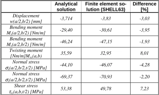
GENERAL POSTPROC / RESULTS VIEWER – selection of the component 13.3 Comparison of the results by analytical and finite element solutions
The results obtained from the two different solutions are listed in Table 13.4. The dis- placement, bending moment and the normal stresses were calculated in the midpoint of the plate, the twisting moment and shear stress were determined at the corner point, respec- tively. Based on the table it is seen that there is a very good agreement between the ana- lytical and finite element solutions. In each case the result by finite element solution is higher than that obtained from analysis, except for the case of the twisting moment and the shear stress.
Analytical solution
Finite element so- lution (SHELL63)
Difference [%]
Displacement
w(a/2,b/2) [mm] -3,714 -3,83 -3,03
Bending moment
Mx(a/2,b/2) [Nm/m] -29,40 -30,61 -3,95
Bending moment
My(a/2,b/2) [Nm/m] -46,24 -47,15 -1,93
Twisting moment
[Nm/m]Mxy(a,b) 35,59 32,95 8,01
Normal stress
σx(a/2,b/2,t/2) [MPa] -44,10 -46,07 -4,28
Normal stress
σy(a/2,b/2,t/2) [MPa] -69,37 -70,93 -2,20
Shear stress
τxy(a,b,t/2) [MPa] 53,38 49,78 7,23
Table 13.4. Comparison of the solutions by analytical and finite element calculations.
13.4 Bibliography
[1] S. Timoshenko, S. Woinowsky-Krieger. Theory of plates and shells. Technical Book Publisher, 1966, Budapest (in hungarian).
[2] J.N. Reddy, Mechanics of laminated composite plates and shells – Theory and ap- plications. CRC Press, 2004, Boca Raton, London, New York, Washington D.C.
[3] ANSYS 12 Documentation. http://www.ansys.com/services/ss-documentation.asp.