CHAPTER THREE
SOME ADDITIVE PHYSICAL PROPERTIES OF MATTER
3-1 Introduction
In this chapter we take up a number of physical properties of matter, especially of liquids and gases, which are useful and important to know about but whose detailed theory is somewhat specialized for a text at this level. In contrast to Chapter 2, then, the present chapter will be in a somewhat descriptive vein.
The properties to be discussed have an aspect in common. They arise from the interaction of an electric or magnetic field with molecules and, to the first approxi
mation, are determined by the separate behavior of atoms or small groups of atoms within a molecule. As a consequence the properties are approximately additive. By this is meant that the molar value of the property, which is what is measured experimentally, can be formulated as a sum of contributions from various parts of the molecules present. The presence of additivity on a molecular scale means also that the value of the property for a mixture of species will be additive.
To be more specific, if & denotes the molar property, then if the molecular formula is AaB&Cca d d i t i v i t y means that
& = a & A + b &B + c0>c + - , (3-1) where ^ A and so on denote the atomic properties. For a mixture of species the
average molar property is
= l ~F~ Χ<ιβ*2 "Τ" *'* = Σ i ' (3~2)
i
where ^f is the molar property of the ith species and χ denotes mole fraction. This last attribute becomes very useful in that, by means of the physical measurement, one may determine the composition of a mixture or, as in chemical kinetics, follow changes in composition with time.
We have already encountered some additive properties. Mass is strictly additive (neglecting relativity), so molar mass or molecular weight obeys Eqs. (3-1) and (3-2) exactly. Volume at constant pressure and temperature is additive, but usually only very approximately so in the case of liquids. The properties to be taken up here will similarly be at least approximately additive.
75
The Commentary and Notes section of this chapter is devoted to a discussion of the cgs and the SI (or mksa) systems of units.
The term "light" will be used in the present context to mean electromagnetic radiation generally. That is, the radiation need not be of wavelength corresponding to the visible region: It could be ultraviolet, infrared, or microwave radiation.
Such radiation can interact with matter to show various effects such as refraction, scattering, and absorption. It is only the last that we discuss at the moment. The phenomenon of optical activity is taken up in Section 19-ST-2.
When light is absorbed its energy is converted into some other form, and we accept that this conversion can only occur in the discrete amount given by the quantum of energy of the light. It is part of the quantum theory of light that this quantum of energy is given by hv, where h is Planck's constant and ν is the frequency of the light. The usual consequence of absorption of a light quantum is that some particular molecule gains energy hv and is thereby put in some higher energy state, that is, in some excited state.
A point of importance here is that although light can only transfer energy in units of quanta, it otherwise behaves as a wave. One consequence is that the train of waves passing through a region of matter may or may not interact with any of the molecules present. There is only a certain probability that interaction will occur.
The derivation of the absorption law is then based on a probability analysis.
Let kx be the probability that light of a given wavelength will be absorbed per unit length of matter; kx8 is then the probability of absorption in some small distance δ. The probability that the light is not absorbed is 1 — kx8. Further, the probability that light will not be absorbed in a second increment of distance δ is (1 — kxS)2 and the probability of its not being absorbed in η such distances be
comes (1 — kxS)n.
Now let χ be the total distance, χ = n8. We want to keep the same path length x9
but to take the limit of η o o , that is, the limit of an infinite number of infinites
imal lengths δ:
I It should be recognized that lim/ |_^c o[l + (1 /n)n] = e.\ The probability that light will not be absorbed in distance χ is then e~kxx. If light of intensity I0 is incident on a portion of matter, then the probable intensity after a distance χ is
I/I0 is the fraction of light transmitted through, that is, not absorbed by, a sample of thickness x.
Equation (3-4) is a statement of Lambert's law, where kx is the linear absorption coefficient (also called the Napierian extinction coefficient b). However, since the absorption process is a molecular one, it is somewhat more rational to recognize that, per unit area of target, a depth / will contain lp/m molecules, and to write Eq. (3-4) as
3-2 Absorption of Light
(3-3)
/ = I0e (3-4)
kxm
Ρ (3-5)
3-2 ABSORPTION OF LIGHT 77 where ρ and m are respectively the density and the mass per molecule of the material, Ν is the number of molecules traversed per square centimeter, and kN is now the molecular absorption coefficient.
An important special case is that in which the absorbing species is present in solution. If we can assume that kN is not affected by concentration, then, since Ν = N0ClΊ'1000, where C is in moles per liter, that is, in units of molarity Af,
{ = — τ & · <M>
The constant α is called the molar absorption coefficient, and Eq. (3-6) is a statement of the combined Beer-Lambert law for light absorption.
Finally, a common modification of Eq. (3-6) is
I0 ' 2.303 ' V }
If we now define the optical density D as equal to log(/0//), we have
D = eCl. (3-8) The quantity D is alternatively called the absorbance and is denoted by the
symbol A. Also, the extinction coefficient e is alternatively called the molar absorp
tivity.
Returning to the derivation that led to Eq. (3-3), if more than one type of interacting species is present, then the probability kx of absorption per unit distance will now be given by a sum over all species, kXttoi = Σ kx.i · The same applies to the other absorption coefficients. In particular, for a solution of more than one species, we get
Λ =
/ Σ « Λ .
(3-9)Often the product e/C for the solvent is abstracted from the sum to give
D = D.+ (3-10) Optical density or absorbance is thus an additive property of mixtures, to the
extent that changing concentration does not change the character of the species present. It may also be additive with respect to chromophoric groups within a molecule; this is especially common in the case of infrared spectra where vibrational excitations of the various types of bonds contribute somewhat independently to the overall absorption. It should perhaps be emphasized that e is very much a function of wavelength so that any statement of an e value must be accompanied by the wavelength to which it pertains.
Example. A 0.01 Μ solution of C r ( N H8)6( N C S )2 + (as the perchlorate salt) absorbs 88.79%
o f incident light o f 5 0 0 n m wavelength w h e n placed in a 1-cm spectrophotometer cell. T h e solvent m e d i u m absorbs s o m e w h a t at this wavelength; a 10-cm cell filled with solvent transmits 31.6% of incident light at 5 0 0 n m .
O n standing, the reaction
C r ( N H3)6( N C S )2+ + HaO = C r ( N H3)5( H20 )3 + + N C S "
A Β
occurs and the reaction goes t o completion in several weeks at 45°C. The per cent transmission of this final solution through a 1-cm cell is 44.64. H o w far had the reaction proceeded after 75 hr at 45°C if, after this time, the optical density of the solution in the 1-cm cell was 0.650? A l s o calculate the extinction coefficients of the complex ions A and B.
First, the various statements should be reduced to optical densities for a 1-cm path length.
For the original solution, D0 = l o g ( /0/ / ) = - l o g (0.1121) = log (8.92) = 0.950. For the solvent, De = - l o g ( 0 . 3 1 6 ) = log(3.16) = 0.500, or, for a 1-cm path length, DB = 0.050. The net optical density due to the starting complex is then 0.950 — 0.050 = 0.900, and the extinction coefficient is therefore eA = 0.900/0.01 = 90.0 liter m o l e- 1 c m- 1. After complete reaction, Doo = —log(0.4464) = log(2.24) = 0.350. The net optical density due to the product is then 0.350 - 0.050 = 0.300 and the extinction coefficient of the product is cB = 0.300/(1 χ 0.01) = 30.0 liter mole"1 c m "1.
The net optical density after 75 hr is 0.650 - 0.050 = 0.600. Then, by Eq. (3-10) 0.600 = (1)(90.0CA + 3 0 . 0 CB) = 6 0 . 0 CA + 0.300
(since CB = 0.01 - CA) , or CA = 0.300/60.0 = 0.0050 M. The reaction had thus proceeded to 5 0 % , or by one half-life.
3-3 Molar Refraction
A second type of interaction of light with a medium is refraction, measured by the index of refraction «, which gives the ratio of the velocity of light in vacuum to that in the substance. The actual experimental measurement is based on the bending of a light ray as it passes from air into the medium.
The theory involves the interaction of the oscillating electric field of electro
magnetic radiation with the various characteristic frequencies for electrons in an atom or collection of atoms, and leads, in first order, to the equation
where the sum is over the various characteristic frequencies v0 for a given frequency of radiation v. Ordinarily, ν is small compared to any v0, so the index of refraction does not vary much with the wavelength of light used, although for η to be purely characteristic of the atom, ν should be zero. Often, however, a standard wavelength, such as that of the yellow emission from a sodium lamp, is used.
There is an important exception to this situation. If the compound absorbs light this means that there is some transition between states of differing energy. This energy corresponds to a frequency hv0 and, as a consequence, the index of refraction will vary rapidly as the frequency of the light used, v, is varied through the value of v0, that is, through a region of strong light absorption. For most small molecules, however, vQ is rather large; in fact, hvQ often corresponds approximately to the ionization energy of the molecule.
An early treatment by H. A. Lorentz and L. V. Lorentz in 1880, as well as more modern ones, considers that the index of refraction should vary with the density of a medium of given atomic composition according to the relationship
n*- \ Μ
Here M/p is the molar volume and R is a quantity called the molar refraction. If molecules are treated as perfectly conducting spheres and light of infinite wavelength is used in measuring «, then R is the actual molar volume of the molecule.
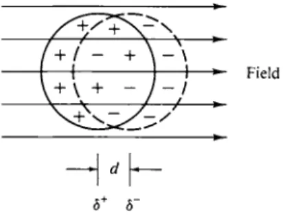
3-3 MOLAR REFRACTION 79 There is an alternate way of treating this limiting situation. An imposed electric field F will in general displace the electrons in an atom somewhat to produce a dipole moment as illustrated in Fig. 3-1. A charge separation occurs in the initially
FIG. 3 - 1 . Molecular dipole moment induced by an electric field.
Field
δ+ δ~
electrically symmetric atom, equivalent to having small equal and opposite charges 8+e and 8~e separated by distance d. The dipole moment μ is defined as
μ = 8ed, (3-13) where e is the charge on the electron. The traditional unit for dipole moment is the
debye (D), defined as 1 0- 1 8 esu cm. Since d is of the order of 1 A and e has the value 4.803 X 10~1 0 esu, dipole moment quantities generally come out as some small number of debye units. (In the SI system, dipole moment is given in coulomb- meter units.)
The induced dipole moment is proportional to the electric field,
/*ind = ma = aF, (3-14)
where the proportionality constant α is called the polarizability and the symbol m is used for moments induced by various individual effects. Only one such effect is present in Eq. (3-14), so that here μ1 η ά and ma are the same. The symbol μ is reserved for the experimentally observed dipole moment; if it is induced, the subscript " i n d "
may be used. In general, / xi n d may be the sum of more than one term [as in Eq. (3-18)]. In the cgs system, the field is in esu per centimeter squared, the dipole moment in esu-centimeter, and α is then in cubic centimeters. Usual values of α are about 1 0 "2 4 c m3 or about actual atomic volumes. (In the SI system, polariza
bility has the dimensions of coulomb square meter per volt and F of volts per meter. Alternatively, polarizability has the units of e0 m3 where e0 is the permit
tivity of vacuum, 8.842 χ 1 0 "1 2. (See Section 3-CN-l.)
The conducting sphere model provides a connection between index of refraction at infinite wavelength, [v = 0 in Eq. (3-11)] and the polarizability of the sphere, again given by Lorentz and Lorentz. This relationship is
η2 — \ Μ 4
R» = ^ + I 7 = ^ a ' ( 3"1 5 )
where N0 is Avogadro's number. Thus α corresponds to the cube of the radius of the sphere.
As suggested by the summation of Eq. (3-11), molar refraction is, ideally, an additive property; empirically, it is very nearly one. Thus values of R can be
assigned to individual atoms in an organic molecule. Somewhat better results are obtained if molar polarizations are assigned to types of bonds rather than to in
dividual atoms. See Glasstone (1946) and Moelwyn-Hughes (1961).
Example. Calculate the molar refractions for t w o isomeric liquids at 2 0 ° C , acetic acid and methyl formate. T h e respective molar v o l u m e s M/p are 60.05/1.0491 = 57.24 c m8 m o l e "1 and 60.05/0.9742 = 61.64 c m3 m o l e "1; and the refractive indices with the s o d i u m D line are 1.3721 and 1.3433, respectively. Substitution into Eq. (3-12) gives molar refractions o f 13.013 c m8 m o l e "1 for acetic acid and 13.033 c m8 m o l e "1 for methyl formate. T h e respective values from the atomic refractions are 12.972 and 13.090 c m3 m o l e "1 (and those from the b o n d refractions, 12.770 and 12.782 c m3 m o l e "1, but n o w for infinite wavelength).
3-4 Molar Polarization; Dipole Moments
It was stressed in the preceding section that, on theoretical grounds, the index of refraction should be for zero-frequency light in the calculation of molar refraction. As an alternative, one may directly impose an external low- or zero- frequency electric field on the medium by having it between the plates of a capacitor.
The capacity of a parallel plate capacitor is
c
= ¥ = % =
C>
D> ™
where q and Ε denote the charge on each plate and the effective field between them, respectively. (In this section we use Ε to denote an applied field and F to denote the actual local field experienced by a molecule; both are expressed in volts per centimeter.) In the presence of a medium other than vacuum, the effective field, instead of being equal to E0 , the applied potential difference, is reduced to E0/Z>, where D is the dielectric constant. The effect is to increase C over the value for vacuum C0. The value of C0 is related to the dimensions of the capacitor,
Q = < £ . (3-17) where srf is the area of the plates and d their separation.
From a molecular point of view, the presence of the field induces a proportional dipole moment in the molecules as in Eq. (3-14). At the low frequencies which characterize dielectric constant measurements there are now two (main) contri
butions to / xi n d . As before there is the dipole moment arising from the polarizability of the molecule, ma, and there is also the effective moment mu resulting from the partial net alignment by the field of any permanent molecular dipoles that are present. This second type of induced dipole moment is again proportional to the field acting on the molecules (as discussed later) and the proportionality constant
is called the orientation polarizability αμ . Equation (3-14) becomes
/^ind(tot) = M< * + M/ X = 0 * + aJ F (3-18) or
mtot = <*totF. (3-19)
3-4 MOLAR POLARIZATION; DIPOLE MOMENTS 81
or, from Eq. (3-20), remembering that E0 = £>E,
F = \{D + 2)E. (3-22) On eliminating E, we obtain
3 \ 4 w 4
F(* ~D^l) = 3π 1 = 3πίΆίοΐη>
and, on eliminating F by means of Eq. (3-18), we obtain D- 1 4
D + 2 = 3 7 r n at o t . (3-23)
Since η = N0p/M, the final form is
Ρ is called the molar polarization and the contribution to Ρ from the polarizability α of the molecules is denoted Pa. Theoretical analysis shows t h a t Pa should be equal to R, the molar refraction, provided the latter is the limiting value from indices of refraction at infinite wavelength, R0.
The contribution of αμ [Eq. (3-18)] to the total polarizability is quite important if the molecules have a nonzero dipole moment μ. This will be the case if bonds between unlike atoms are present, as in N O or HC1, provided there is no internal cancellation of such bond dipoles, as happens in C H4 or C 02 owing to molecular symmetry. The relationship between ocu and the permanent molecular dipole moment μ is as follows.
If a molecule has a permanent dipole moment, it will tend to be oriented along the direction of the local electric field F. That is, the energy € of the dipole in the field would be zero if it were oriented perpendicular to the field and it would be μ¥
if it were oriented in line with the field. For some intermediate orientation
€ = ¥μ C O S 0, (3-25)
If the molecules are far apart, as in a dilute gas, the total induced polarization simply acts to reduce the apparent field E0; from an analysis of the situation using Eq. (3-17) one finds
Ε = E0 - 4TTI, (3-20) where I is the total polarization per unit volume, I = mt o tn and η denotes concen
tration in molecules per cubic centimeter.
More generally, however, the degree of polarization of each molecule is affected by the field of the induced polarization of the other molecules, and it is necessary to take this into account. This corrected, or net effective local field F is now given by
F = Ε + ΙττΙ, (3-21)
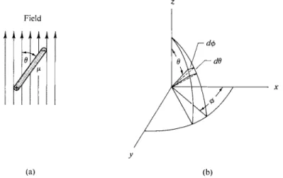
where, as shown in Fig. 3-2(a), θ is the orientation angle defined such that μ cos θ gives the component of μ in the field direction. At 0 Κ all dipoles should orient completely, but at any higher temperature thermal agitation will prevent this and the probability of a given orientation is proportional to the Boltzmann factor e-€lkT. At infinite temperature the effect of the field becomes negligible; all orientations are then equally probable and the average net dipole moment of a collection of molecules is zero.
What is now needed is the average orientation or, more precisely, the average of μ cos Θ, which gives the average net dipole moment mu. The procedure followed is that discussed in Section 2-4; that is, one writes the averaging equation
_ Ν $£(μ cos θ) e-<fmcos0)/fcr(277 sin β αβ)
m" " ^ j je- ( f m c o s 0) /f cr (2 7 r sinflrffl) ' ( " } where Ν is the number of molecules and (2 π sin θ άθ) gives άω, the element of solid angle.
In the polar coordinate system used (shown in Fig. 3-2b) an element of solid angle is given by
άω = sin θ άθ άφ.
Integration over all directions gives
άω = sin θ άθ άφ = | - c o s θ \ \ φ | =4 π. (3-27) j 0 j 0 ο ο
In the present case the energy is not affected by the φ angle, so this is integrated out in Eq. (3-26) to give the factor 2π.
The integrals of Eq. (3-26) may be evaluated as follows. Let a = μΈ/kT and χ = cos 0, so ax = sin θ άθ; then
ΗΙΜ _ ^eaxxax μ J"1 eax ax
FIG. 3-2. (a) Component of dipole moment in the direction of a field, (b) Polar coordinate system.
3-4 MOLAR POLARIZATION; DIPOLE MOMENTS 83 60
50
_ 40
"o
ε
"B 30
20
10
C H3C 1 /
/ N H3
' HC1
" / /
HI1 1 1 1 0 1 2 3 4 5
1 03/ Γ
FIG. 3 - 3 . Variation of molar polarization with temperature.
The integrals are now in a standard form, and algebraic manipulation gives+
ΠΐΜ — = coth a , (3-28)
Under ordinary experimental conditions μΈ/kT is small compared to unity, and on expansion of the expression (coth a — I/a), the first term is a/3. To a first approximation we have
m
« = ( w )
F- <
3-
29>
Comparison with Eq. (3-18) gives
μ*
OL = — -
3kT
The expression for Ρ [Eq. (3-24)] may now be written explicitly as
4 4 u2
(3-30)
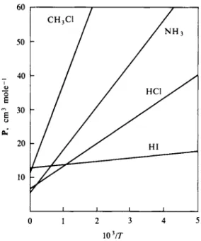
(3-31) Thus the molar polarization Ρ as obtained from dielectric constant measurements should vary with temperature according to the equation
b 4 4 u2
Ρ = a + ψ , where a = Pa = R0 = j TTN0OC, b = j πΝ0 . (3-32) Equation (3-32) is known as the Debye equation, and typical plots of Ρ versus l/T are shown in Fig. 3-3,. Equation (3-32) is valid for gases. In liquids, especially associated ones, the molecular dipoles may not be able to respond freely to the applied field.
+ cosh χ = \{ex + e~x) and sinh χ = %(ex — e~x); coth χ = (cosh x)/sinh x.
Example. S o m e sample calculations are n o w in order. First, the statement that Έμ/kT is ordinarily a small quantity c a n b e verified. A capacitor might b e charged t o as m u c h as 6 0 0 0 V c m- 1, or t o 6 0 0 0 / 3 0 0 V esu c m- 1. Taking this a s the approximate local field F , a n d taking μ to b e in the usual range o f about 1 0 "1 8 esu c m , w e h a v e
€ = 1 0 " 1 8^ = 2 χ 1 0 - " erg.
If Γ is about 300 K, then kT is (1.38 χ 1 0 "1 β) ( 3 0 0 ) or about 4 x 1 0 "1 4 erg. T h e n e/kT is a b o u t 5 x 1 0 "4, and is indeed a small number.
This calculation m a y also b e m a d e in the SI system (see C o m m e n t a r y a n d N o t e s ) . N o w F is 6 0 0 0 V per 0.01 m or 6 χ ΙΟ5 V m_ 1. A dipole m o m e n t o f 1 0 "1 8 e s u c m n o w has the value
1 0_ 1 8/ 1 0 c C meter, where c is the velocity of light, used here as 3 χ 1 01 0c m s e c_ 1; μ is thus
1 χ jo-2 9 Q m et e r . T h e energy of the dipole in the field is still μ¥, and has the value (6 χ 105)
(i) x 1 0 ~2 9o r 2 χ 1 0 "2 4 J (joule); the B o l t z m a n n constant is n o w 1.38 x 1 0 ~2 8 J K_ 1, s o kT b e c o m e s 4 χ 1 0 "2 1 J. T h e ratio c/kTis then 5 χ 1 0 "4, as before.
Turning next to an application of the D e b y e equation, w e find that the dielectric constant of gaseous HC1 at 1 atm pressure is reported (International Critical Tables) to be 1.0026 at 100°C and 1.0046 at 0°C. T h e molar volume RT/P is then 30.62 and 22.41 liter m o l e- 1 at the t w o tem
peratures, respectively. T h e corresponding Ρ values are, f r o m Eq. (3-24), 26.51 c m8 m o l e- 1 a n d 34.31 c m8 m o l e- 1. T h e straight line through these t w o points o n a plot of Ρ versus l/T gives a n intercept a = 5.21 a n d slope b = 7.95 χ 1 08.
F r o m Eq. (3-32), α = (3)(5.21)/(4)(3.141)(6.023 χ 1 02 8) or a = 2.07 χ 1 0 "2 4 c m8 (a better value is 2.56 x 1 0 "2 4) . W e also have μ2 = (9)(1.38 χ 1 0 "1 β) ( 7 . 9 5 χ 108)/(4)(3.141)(6.023 x 1 02 8) or μ2 = 1.30 χ 1 0 "8 β a n d μ = 1.14 D (debye). This calculation, while illustrating the use o f the D e b y e equation, gives s o m e w h a t approximate values for a a n d μ because o f the inaccurate evaluation o f a a n d b from just t w o points (a better value is 1.05 D ) .
Dipole moments may also be determined from measurements at a single temperature if a dielectric constant measurement is combined with one of index of refraction. The latter gives the molar refraction and hence Pa directly, for use in Eq. (3-32). Indices of refraction, however, are usually measured with visible light, as with the sodium D line, and some corrections are necessary to convert the value of R so obtained to R0 .
This general approach m a y b e extended t o solutions. T h e molar polarization o f a solution is a n additive property, s o that for a solution
p _ D - l XlMl + XlM2 = + x ^
D + 2 ρ
where χ denotes m o l e fraction. Px is obtained from measurements o n the pure solvent a n d P2 can then b e calculated for the solute. T o discount s o l u t e - s o l u t e interactions, the resulting P2 values are usually extrapolated t o infinite dilution. T o obtain R2, o n e applies the same pro
cedure t o molar refractions from index o f refraction measurements and then proceeds as before t o calculate a dipole m o m e n t for t h e solute. N o t only is this procedure s o m e w h a t approximate, but the solvent will often have a polarizing effect o n the solute as a result o f solvation interactions. Consequently P2 a n d corresponding μ values will n o t in general b e exactly the s a m e as those obtained f r o m the temperature d e p e n d e n c e o f the dielectric constant of the pure solute vapor. In the case o f nonvolatile, solid substances, however, the solution procedure m a y b e the best o n e available for estimating molecular dipole m o m e n t s .
3-5 Dipole Moments and Molecular Properties
It is conventional and very useful to regard a molecular dipole moment as an additive property. One assigns individual dipole moments to each bond and the addition, of course, is now a vectorial one.
In the case of diatomic molecules the bond moment is just the measured dipole moment of the molecule. One can proceed a step further. If the internuclear distance
3-5 DIPOLE MOMENTS AND MOLECULAR PROPERTIES 85
T A B L E 3-1. Dipole Moments and Polarizabilitiesa
Polarizability D i p o l e m o m e n t
Substance
(A
3)
( D )H e 0.204 —
A T 1.62 —
H2 0.802 —
N2 1.73 —
C I , 4.50 —
HC1 2.56 1.05
HBr 3.49 0.807
H I 5.12 0.39
co
2 2.59 0.00HzO 1.44 1.82
N H3 2.15 1.47
CH3C1 — 1.87
C e H6 25.1 0.00
CeH5C l — 1.70
/ ? - CeH4C l2 — 0.00
<?-CeH4Cl2 — 2.2
AW-CeH4Cl2 — 1.4
α F r o m R0 values.
is known from crystallographic or spectroscopic measurements, then from the definition of dipole moment μ = bed [Eq. (3-13)], the fractional charge Se on each atom can be calculated. This is, in effect, the degree of ionic character of the bond.
Some dipole moment values are given in Table 3-1 and the calculation may be illustrated as follows. The bond length for HC1 is 1.275 A and the dipole moment is 1.05 D (debye). The fraction of ionic character δ is then 1.05 χ 10"1 8/(1.275 χ 10"8)(4.80 χ 10"1 0) = 0.17. The H - C l bond is thus said to have 1 7 % ionic character. The similarly obtained values for H F , HBr, and HI are 45 %, 11 %, and 4 %, respectively. This set of values has been used to relate the electronegativity difference between atoms and the degree of ionic character of the bond [see, for example, Douglas and McDaniel (1965)].
Turning to triatomic molecules, Table 3-1 shows a zero dipole moment for C 02. This is not because the individual C=0 bonds are nonpolar, but because the two bond dipoles cancel, as illustrated in Fig. 3-4(a). This arrangement of two dipoles end-to-end corresponds to a quadrupole (see Special Topics) and the experimental quadrupole moment of —4.3 X 10~2 6 esu c m2 for C 02, when combined with the
26"
(a) (b) F I G . 3-4. (a) A molecule with zero dipole moment (but nonzero quadrupole moment), (b) Vector addition of bond dipole moments for water.
T A B L E 3-2. Some Bond Dipole Moments*
Bond M o m e n t ( D ) B o n d M o m e n t ( D )
O - H - 1 . 5 3 C - C l 1.56
N - H - 1 . 3 1 c - o 0.86
C - H ( - 0 . 4 0 )b 2.4
C - F 1.51 3.6
° The sign of the dipole m o m e n t indicates that of the first-named atom.
b Assumed value.
known C = 0 distance, indicates that each oxygen atom carries a charge of about 0.3e.
Water, on the other hand, shows a net dipole moment because the bond angle is not 180° and the two Η—Ο dipoles fail to cancel. As illustrated in Fig. 3-4(b), the actual angle is 105° and the observed moment is the vector sum of the two bond moments.
The situation becomes increasingly complicated with polyatomic molecules. The net dipole moment of ammonia is now the vector sum of three Ν — Η bond moments, while for the planar B F3 molecule the three bond moments cancel to give zero molecular dipole moment. The same cancellation occurs for C H4, which is unfortunate, since one thus gets no information about the C—Η bond moment.
An indirect estimate (Partington, 1954) gives —0.4 for ^C_H (carbon is negative), and this now permits the calculation of other bond moments involving carbon.
Thus μο-ci can now be obtained from the dipole moment of CH3C1 and a knowledge of the bond angles.
A few such bond moments are collected in Table 3-2. It must be remembered, however, that the resolution of a molecular moment into bond moments is somewhat arbitrary. Thus one could assign a moment to the lone electron pairs in water or ammonia as well as to the bonds. Also the dipole moment of a molecule is merely the first term in an expansion of the function which describes the complete radial and angular distribution of electron density in a molecule (see Special Topics).
This function, however, is in general not known or can only be estimated theoret
ically, and the bond moment procedure just given is adequate for many purposes.
Finally, molecular dipole moments can provide useful qualitative information.
Thus the zero moment for /?-C6H4CI2 must mean that the C—CI bonds lie on the molecular axis, while the nonzero moment for /?-C6H4(OH)2 (of 1.64 D) indicates that the Ο—Η bonds lie out of the plane of the ring. The series of ρ-, m-, and 0-isomers of C6H4C 12 can be identified since the order given should be that of increasing dipole moment. As an example from inorganic chemistry, the isomers of square planar P t A2B2 complexes can be distinguished on the basis of their dipole moments. That of the trans isomer should be small or zero, whereas that of the cis isomer should be fairly large. As a specific example, the isomers of Pt[P(C2H5)3]2Br2 have dipole moments of zero and 11.2 D.
Interatomic distances in a molecule may also be determined by x-ray diffraction studies on crystals (Chapter 20), electron diffraction studies on gases (Section 20-CN-1C), infrared spectroscopy (Section 19-5), and microwave spectroscopy (Section 19-CN-l).
COMMENTARY AND NOTES, SECTION 1 87
COMMENTARY AND NOTES 3-CN-l Systems of Units
It is appropriate to comment at this point on the rather mixed state of affairs in the matter of systems of units [see Adamson (1978)]. The standard metric or cgs system leads to the erg and the dyne as the units of energy and of force, respec
tively, and through the mechanical equivalent of heat, to the calorie as an alterna
tive unit of energy. Force is defined by means of Newton's first law,
f=ma9 (3-34)
where a denotes acceleration, and the dyne is that force required to accelerate 1 g by 1 cm s e c "2. The dimensions of dyne and erg are g cm s e c "2 and g c m2 s e c "2, respectively. The unit of volume is the cubic centimeter, with the liter or 1000 c m3 as a secondary unit.
The mks (meter-kilogram-second) system, now incorporated by a set of inter
national commissions into what is called the SI system (Systeme Internationale d'Unites) makes several changes. The unit of force is still given by Eq. (3-34), but in terms of kg m s e c "2, and is now called the newton (N). One Ν is 105 dyn. The unit of energy is in kg m2 s e c "2, or the joule (J). One J is 107 erg. (See McGlashan, 1968.)
In addition to critically reevaluating the numerical values of fundamental con
stants, the SI commissions recommended that use of the calorie be dropped, as well as special names for subunits such as the liter, micron ( 1 0 "6 m), and angstrom ( 1 0 "8 cm). A special set of prefixes was adopted for the designation of multiples or fractions of the primary units. These are tabulated on the inside cover. For example, nano- means 1 0 "9 and the closest SI unit to the angstrom is the nano
meter (nm) or 1 0 "7 cm.
Avogadro's number was not changed, however, and molecular weights therefore have changed. Thus the molecular weight of 02 is 0.03200 kg m o l e "1 in the SI system.
At the time of this writing the cgs and related conventional units remain in principal usage in U.S. technical journals in chemistry, although our National Bureau of Standards has supported use of the SI system. Great Britain officially requires the use of SI units in British journals; usage is mixed in other European countries. Textbooks of physical chemistry in the United States are now recognizing both systems, as is done here. There appears to be a slow movement toward com
plete adoption of the SI system.
Since this is a commentary section, an opinion is permissible. The cgs system and associated secondary units have three important characteristics. (1) It is decimalized (unlike the English units such as feet and inches). (2) Units are defined operationally, that is, in terms of fundamental laws such as Newton's law. (3) Com
monly measured quantities come out to be of the order of unity. Thus the density of water is about 1 g c m "3 and its heat capacity about 1 cal g "1 K "1; the size of an atom is about 1 A ; pressure at sea level is about 1 a t m ; the molecular weight of hydrogen is about 1 g m o l e "1, and so on.
The SI system retains (1) but departs from (2) (discussed later) and (3). With respect to (3), for example, the density of water becomes about 1 03k g m ~3 (or 10 " 3 kg cm " 3) , and its heat capacity about 4 χ 1 0eJ K ~1m- 3; atoms are around 0.1 nm in size; sea level pressure becomes about 1 χ ΙΟ5 Ν m "2; the atomic weight of hydrogen is 10 "3 kg mole "1.
Criterion (3) alone suggests that the cgs and related units will continue to be used. Convenience is important in science as it is elsewhere. (Consumers in the United States are being urged to think in terms of liters rather than quarts; they will be yet more reluctant to buy milk in terms of cubic meters or decimeters or to joule-count in watching their diet!)
The situation with respect to electrical and magnetic units is as follows. In the cgs system the fundamental law of electrostatics is Coulomb's law,
/ = £ · (3-35) The unit of electrostatic charge, the esu or statcoulomb, is defined operationally by
the statement that unit charges repel each other with a force of 1 dyn if at a distance of 1 cm apart. (Coulomb's law is central to chemistry in many ways, but perhaps most importantly in being basic to quantum theory and wave mechanics.) If the medium is other than vacuum, the force is reduced by the factor D,f = q2\Dr2>
where D is the dielectric constant of the medium.
Similarly, in electromagnetics, unit magnetic poles repel with a force of 1 dyn if separated by 1 cm; magnetic field intensity Η is 1 Oe (oersted) if unit magnetic pole placed in it experiences a force of 1 dyn. Both definitions are for vacuum. The field in a medium is reduced from that in vacuum by the magnetic permeability μ.
Current, i, in the esu system is just the number of esu per second or statampere;
it is thus a secondary unit. In the emu system, however, current is defined opera
tionally as that current which in a single-turn circular loop of wire of 1-cm radius produces a magnetic field intensity of 2π Oe. The unit of current is the absolute ampere or abampere. Our practical, everyday ampere, A, is 0.1 abampere. Also, because of the differences in operational definition, 1 abampere = c statampere, where c is the velocity of light.
In the emu system, charge is defined as abamperes χ seconds; the unit is the abcoulomb. The practical coulomb, C, is 0.1 abcoulomb. Also, the abcoulomb or emu unit of charge is c statcoulombs or esu units of charge. Thus the charge on the electron is 1.602 χ 1 0 -2 0e m u , 1.602 X 1 0 "1 9C , and 4.802 χ 1 0 -1 0e s u .
Finally, potential is defined in terms of the work required to transport unit charge. Unit potential difference exists between two points if 1 dyn is required to transport unit charge. If the charge is 1 esu, the potential is 1 statvolt; if the charge is 1 emu, the potential is 1 abvolt. The practical volt, V, is defined separately as requiring 1 J for the transport of 1 coulomb. It follows that 1 V is 108 abvolt and 1/300 statvolt.
The SI system uses only the practical set of units, A, C, and V. The four funda
mental quantities are m, kg, sec, and A. There is a problem with Coulomb's law.
A conversion factor is needed if force is to be given in Ν with charge in C and r in m.
Further, since certain equations of electricity and magnetism contain factors of 2π or 4TT [Eq. (3-20) is an example], the restatement of Coulomb's law is so made that such factors do not appear in situations where geometric intuition does not seem
SPECIAL TOPICS, SECTION 1 89
to call for them. The law is written
/ = 4 7 Γ€0Γ (3-36)
where e0 is the permittivity of vacuum and is equal to 107/47rc2 or 8.854 χ 1 0 "1 2 A2 sec4 k g "1 m ~3. A similar redefinition of magnetic interaction requires a magnetic permeability of vacuum, μ0, to be 4π χ 1 0 "7 kg m s e c "2 A "2. Notice that ε0μ0 =
1/c2.
For both reasons (2) and (3) presented earlier, it is likely that Coulomb's law will remain as a fundamental defining law in physical chemistry and that therefore the esu system will retain its current usage. The introduction of ε0 in the SI system is awkward both conceptually and practically. As an example relevant to this chapter, polarizability has the dimensions of c m3 in the cgs-esu system and it is pleasing that actual values are of the order of molecular volumes. In considerable contrast, the SI system gives polarizability the dimensions of €0 m3 or A2 sec4 k g "1 and numerical values are far different from molecular volumes.
Generally speaking, it will be the practice in this text to use esu units where Coulomb's law is fundamental to the topic. In electrochemistry, however, the practical system of electrical units (C, A, V) is the one of traditional convenience.
Since this and the SI system are the same, no problem arises.
3-ST-l The Charge Distribution of a Molecule
The wave mechanical picture of a molecule is that of an electron density distri
bution; the charge density at each volume element (or the probability of an electron in that element) is given by the square of the psi function φ for that molecule.
Recalling the coordinate system of Fig. 3-2, we see that this charge density is in general some complicated function of r, 0, and φ, p(r, θ, φ). Now, just as a wavy line can be approximated by a series of terms in cosines and sines, that is, by a Fourier expansion, so can a function in three dimensions be approximated by an expansion in spherical harmonics. In fact, it turns out that the wave mechanical solutions for the hydrogen atom consist of one or another spherical harmonic (Section 16-7). These are just the s, px , p^ , pz, dz2, dX2_y*, dxy , dxz, dyz, and so on, functions.
An s function is spherically symmetric and is everywhere positive (or, alter
natively, everywhere negative). The sum or integral over a charge distribution given by the s function,
where dr is the element of volume, simply gives a charge qe due to the electron cloud behaving as though it were centered at the nucleus (Fig. 3-5a). The algebraic sum of qe and the nuclear charge gives the net charge q. An atom or molecule whose
SPECIAL TOPICS
(3-37)
charge distribution is given by an s function behaves like a point charge q. The energy of interaction with a unit charge q0 is
e = SU_ = qV. (3-38)
Here V is the potential of the test charge,
V = — . (3-39) r
A ρ function has positive and negative lobes, as illustrated in Fig. 3-5(b). The sum over such a charge distribution is zero according to Eq. (3-37). However, the
FIG. 3-5. (a) Charge distribution according to an s function. A monopole. (b) Charge distribution according to a ρ function. A dipole. (c) Charge distribution according to a dgt function. A quad
ruple.
SPECIAL TOPICS, SECTION 1 91
sum or integral
Ρ =
Σ ί Λ =
\rp(r9e,4>)dT (3-40) is not zero. This now corresponds to a dipole moment. Next* an electron distribution as given by the dz* function looks as in Fig. 3-5(c). There is now no dipole moment, but Q is nonzero as given by
β = Σ = \ r2P(r> 0> Φ) dr, (3-41) where Q is called the quadrupole moment.
Thus for a molecule such as HC1, the first approximation, or s contribution, says the molecule is neutral. The second term in the expansion, or the pz contribution, gives the dipole moment. In this approximation the atoms can be regarded as having net charges δ+ and δ~ separated by the bond distance d. The third term in the series expansion, giving the complete charge distribution, would be the contribution of the d22 term. This recognizes that the electrons are not spherically disposed around each atom, but concentrate to some extent between the atoms, that is, form a bond.
In terms of point charges, a quadrupole consists of two equal, opposing dipoles.
In the case of a neutral diatomic molecule like HC1, the complete charge distri
bution is given by the sum of the dipole and quadrupole contributions. With more complicated molecules yet higher moments would be needed. N o t many quadrupole moments are known; the ones that are have been obtained from analysis of spectroscopic data. A few values are given in Table 3-3.
Equation (3-39) gives the potential F d u e to a point charge. The potential energy of a molecule having a charge, a dipole moment, and a quadrupole moment can be expressed in terms of the electric potential at that point and its derivatives:
T, . dV Ο d2V
or
. _ , f + „ + $ * . (3-43)
It is assumed that the dipole and quadrupole are aligned in the χ direction, and
T A B L E 3 - 3 . Some Quadrupole Moments'1
Quadrupole m o m e n t Substance χ 1 02 β (esu c m2)
H2 0.65
02 - 0 . 4
N2 - 1 . 4
C 02 - 4 . 3
C2He - 0 . 8
C2H4 2.0
α F r o m A . D . Buckingham, R. L. D i s c h , and D . A . Dunmur, / . Amer. Chem.
Soc. 90, 3104 (1968).
3-ST-2 Magnetic Properties of Matter
The magnetic properties of matter are of less general interest to the chemist than are the electrical properties. In some cases, however, important information about the electronic structure of a molecule can be obtained.
We measure a quantity called the molar magnetic susceptibility χΜ , which is rather analogous to molar polarization in the electrical situation. A convenient way of making this measurement is by means of a Gouy magnetic balance, illustrated in Fig. 3-6. An electromagnet establishes a field H0 and one measures
To balance
F I G . 3-6. The Gouy balance.
the resulting change in weight of a sample. The sample is contained in a tube which is suspended between the pole pieces of the magnet, with the bottom of the sample at the centerline. The hollow lower portion of the tube compensates for the action of the field on the tube itself. The suspension is attached to a sensitive balance, and one measures the change in pull that occurs when the magnetic field is turned on.
As illustrated in Fig. 3-7(b) the sample may be diamagnetic, in which case the magnetic field within it is less than H0 and magnetic lines of force deflect away from the sample. Alternatively, as in Fig. 3-7(c), the sample may be paramagnetic and show the reverse effects. In the first case the pull decreases when the field is applied;
and in the second case it increases. A straightforward derivation shows that the change in f o r c e / o n the sample is given by
where <srf is the area of the tube, ρ is the sample density, and Μ is the molecular weight.
From the molecular point of view, χΜ is made up of two contributions: that due to the inherent magnetic polarizability α and that due to the alignment in the field of any permanent magnetic moments present. Just as with dipolar molecules in an dV/dx gives the field F in this direction. The verification of Eq. (3-43) is left as an exercise.
SPECIAL TOPICS, SECTION 2 93
F I G . 3-7. Lines of magnetic force in (a) vacuum, (b) a diamagnetic substance, and (c) a paramagnetic substance.
(b)
electric field, the alignment of permanent molecular moments is opposed by the randomizing effect of thermal agitation. The actual equation is
X M = N0(* + - § £ r ) , (3-45) where μΜ is the permanent molecular magnetic moment.
As in the electrical case α describes the tendency of the applied field to induce an opposing field in an otherwise homogeneous medium. A physical description of the effect is that the applied field causes the electrons of the atoms to undergo a precession; this precession gives rise to an electric current which in turn generates an opposing magnetic field. We call the effect diamagnetism, and report a molar diamagnetic susceptibility N0OL or ΧΑ. Pascal observed around 1910 that Xa' s are approximately additive, although as with molar polarization or refraction, correc
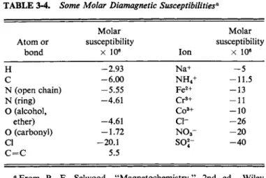
tions are needed for special types of bonds. Some atomic and bond susceptibilities are given in Table 3-4.
A s a numerical illustration, suppose the magnet to provide a field H0 of 10,000 Oe, s/ to be 0.1 c m2, and the sample to consist of water at 25°C. The value of χα for water is —13 χ 10~β and χα(ρΙΜ) is then —0.722 χ 1 0 -ec m -8. Substitution into Eq. (3-44) gives
/ = - J ( 0 . 1 ) ( 0 . 7 2 2 χ 1 0 -6) ( 1 04)2 = - 3 . 6 1 dyn or - 3 . 7 mg.
The force is negative, meaning that the sample will be 3.7 m g lighter when the field is o n .
Permanent magnetic moments arise first of all from the orbital motion of electrons. For a single electron this moment is related to its angular momentum
TABLE 3 - 4 . Some Molar Diamagnetic Susceptibilities'1
Molar Molar
A t o m or susceptibility susceptibility
bond χ 106 Ion χ 10e
Η -2.93 Na+ - 5
C -6.00 N H4+ -11.5
Ν (open chain) - 5 . 5 5 F e2 + - 1 3
Ν (ring) -4.61 C r3 + - 1 1
Ο (alcohol, C o3 + - 1 0
ether) -4.61 c i - - 2 6
Ο (carbonyl) -1.72 N 03- - 2 0
CI -20.1 so2- - 4 0
C = C 5.5
a F r o m P. F. Selwood, "Magnetochemistry," 2nd ed. Wiley (Interscience), N e w York, 1956.
and therefore to the orbital quantum number /, where / = 0 for an s electron, / = 1 for a ρ electron, and so forth. Analysis gives
*
= ( 3-
4 6 )where the quantity (eh/tomc) is known as the Bohr magneton μΒ . Substitution of the numerical values for Planck's constant A, the mass of the electron m, and the velocity of light c gives μΒ = 9.273 χ 1 0 "2 1 erg O e "1 (and 9.273 χ 1 0 "2 4 A m~2 in the SI system).
The second contribution to the permanent magnetic moment is that from the spin of the electron itself. Orbital motion is quantized in units of angular momentum h/2n and spin angular momentum is quantized in units of \Η\2ττ. Since the quantity
\I\2TT appears in both cases, it is not surprising that the spin magnetic moment is related to μΒ :
μΒ = 2μΒ[5(* + 1)]V2, (3.47)
where s is the spin quantum number.
The orbital contribution, Eq. (3-46), is often small; this is because orbital motions of electrons may be so tied into the nuclear configuration of the atom that they are unable to line up with an applied field. As a fortunate consequence only the spin contribution is then important. If more than one unpaired electron is present, the individual spins combine vectorially,
μΒ = 2/xB[5(S + (3-48)
where S is just one-half times the number of unpaired electrons. The molar susceptibility is then
X M = ^ ^ [ 5 ( 5 + 1 ) ] ^ . (3-49) The total observed χΜ is the sum of the negative diamagnetic contribution N0a and
the positive contribution from Eq. (3-49).
Equation (3-49) often applies adequately to elements through the first long row of the periodic table, and therefore allows a determination of the number of unpaired electrons present per molecule. Thus a ferrous compound should have
CITED REFERENCES 95
F I G . 3 - 8 . A modern superconducting magnet installed at the Japanese National Research Institute for Metals. Shown is the N b3S n outer magnet, which gives a central field of 135,000 gauss. With an inner V3G a set of coils, the field becomes 175,000 gauss. In use, the whole unit is immersed in a He cryostat at 4.2K. (Cour
tesy Intermagnetics General Corp.)
four unpaired electrons on the iron and therefore a moment of [2(2 + 1)]1 7VB or 4.90/zB . The observed value is 5.25/xB .
Modern magnetochemistry deals with a great variety of effects in addition t o ordinary susceptibility measurements. These range from studies of transport phenomena in superconductors t o magnetic field effects in spectroscopy. Figure 3-8 shows a contemporary electromagnetic in which superconducting material is used for the coils. This allows very high fields to be obtained with a minimum of energy expenditure (and of heating).
G E N E R A L R E F E R E N C E S HALLIDAY, D . , A N D RESNICK, R. (1962). "Physics." Wiley, N e w York.
SELWOOD, P. (1956). "Magnetochemistry," 2nd e d . Wiley (Interscience), N e w York.
C I T E D R E F E R E N C E S A D A M S O N , A . W . (1978). / . Chem. Ed., 5 5 , 634.
D O U G L A S , Β . E . , A N D M C D A N I E L , D . H . (1965). "Concepts and M o d e l s o f Inorganic Chemistry."
p. 84. Blaisdell, Waltham, Massachusetts.
GLASSTONE, S. (1946). "Textbook o f Physical Chemistry." V a n Nostrand-Reinhold, Princeton, N e w Jersey.
H A N T Z S C H , Α . , A N D D U R I G E N , F . (1928). Z. Phys. Chem. 1 3 6 , 1 .
International Critical Tables, National Research Council, McGraw-Hill, Ν . Y . , 1926-1933.
M C G L A S H A N , M . L. (1968). Physico-Chemical Quantities and Units. Royal Inst, o f Chem. Publ.
N o . 15, London.
M O E L W Y N - H U G H E S , E . A . (1961). "Physical Chemistry." Pergamon, Oxford.