Building Physics
Building Physics
Gudni A. Jóhannesson
TERC Kft. • Budapest, 2013
© Gudni A. Jóhannesson, 2013
End of manuscript / Kézirat lezárva: 2013. január 15.
ISBN 978-963-9968-86-8
Published by TERC Ltd/Kiadja a TERC Kereskedelmi és Szolgáltató Kft. Szakkönyvkiadó Üzletága, az 1795-ben alapított Magyar Könyvkiadók és Könyvterjesztők Egyesülésének
a tagja
A kiadásért felel: a kft. ügyvezető igazgatója Felelős szerkesztő: Lévai-Kanyó Judit
Műszaki szerkesztő: TERC Kft.
Terjedelem: 6,5 szerzői ív
CONTENTS
1. PREFACE ... 13
2. BUILDING PHYSICS ... 15
2.1 What building physics is mainly about ... 15
2.2 Examples of heat and mass transfer ... 16
2.3 Combined processes ... 16
2.4 New mathematical tools make life easier ... 16
2.5 Building physics and the environment ... 17
3. INTRODUCTION TO BUILDING HEAT TRANSFER ... 18
3.1 The basic elements of building heat transfer ... 18
3.1.1 Temperatures ... 18
3.1.2 Heat – a form of energy ... 18
3.1.3 Heat storage – heat capacity ... 19
3.1.4 Energy quality – exergy ... 20
3.1.5 Heat conduction ... 21
3.2 Steady state calculations ... 22
3.2.1 Steady state heat flow and temperature distribution in a multilayer wall with no internal heat sources. ... 24
3.2.2 Surface resistances ... 25
3.2.3 Definition of the U-value ... 26
3.3 Two-dimensional heat conduction ... 26
4. HEAT CONDUCTION EQUATIONS – SIMPLIFICATIONS FOR NON-STEADY STATE SOLUTIONS ... 30
4.1 Simplifications ... 30
4.1.1 No heat production ... 30
4.1.2 No heat production with one dimensional heat flow ... 30
4.2 Solution for a one dimensional slab with harmonic boundary temperatures ... 31
4.2.1 Solution for a multilayer construction ... 34
4.3 Steady state heat flow – simplifications ... 35
4.3.1 Steady state one dimensional heat flow with heat generation ... 35
4.3.2 One dimensional steady state heat flow without heat sources ... 38
5. NUMERICAL METHODS ... 39
5.1 The control element – two dimensional heat flow ... 39
5.2 Expression of boundary conditions ... 42
5.3 Resulting heat balance ... 42
5.4 Choice of time steps and element size – stability ... 43
5.5 Simplifications for special cases ... 43
5.6 Finite element solutions ... 44
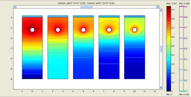
5.6.1 Modelling ground heat exchange with FEM multiphysics ... 45
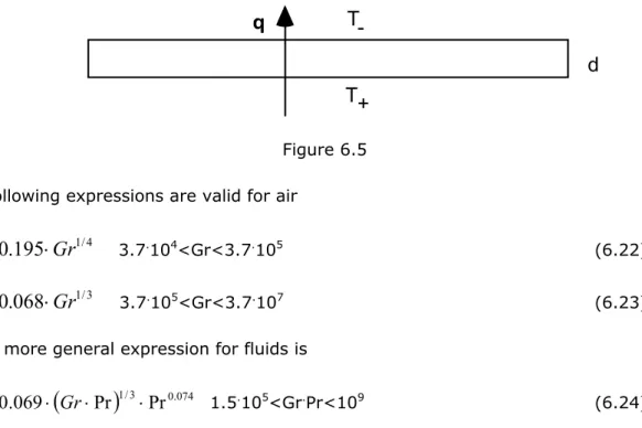
6.1 Basics of convective heat transfer ... 47
6.1.1 Convective surface heat transfer ... 48
6.1.2 Natural convection ... 48
6.1.3 Forced convection ... 48
6.1.4 Dimensionless numbers ... 48
6.2 Expressions for different flow types ... 50
6.2.1 Forced convection ... 50
6.2.2 Natural Convection ... 50
6.3 Expressions for surface heat transfer coefficients ... 50
6.3.1 Forced laminar duct flow ... 50
6.3.2 Forced turbulent flow of air in a duct ... 51
6.3.3 Forced flow along flat surfaces ... 51
6.3.4 Forced laminar flow along a flat surface ... 52
6.3.5 Forced convection with turbulent flow along a flat surface ... 52
6.3.6 Natural convection on room surfaces ... 53
6.3.6.1 Vertical walls ... 53
6.3.6.2 Horizontal surfaces ... 53
6.3.7 Natural air convection within an enclosure ... 54
6.3.7.1 Horisontal gap with upwards heat flow ... 54
6.3.7.2 Vertical gap with limited height H and horizontal heat flow ... 55
6.4 Air flow through building components ... 55
6.4.1 Air flow through an opening ... 56
6.4.2 Air flow through an orifice plate ... 58
6.4.3 Air flow through porous materials ... 59
7. RADIATIVE HEAT TRANSFER – LONG WAVE RADIATION ... 60
7.1 Exemplification of applications ... 60
7.2 Basic theory ... 61
7.2.1 Thermal radiation ... 61
7.2.2 Black body radiation ... 61
7.2.3 Gray body properties ... 62
7.2.3.1 Emissivity ... 62
7.2.3.2 Total absorptance ... 62
7.2.3.3 Total reflectance ... 63
7.2.3.4 Total transmittance ... 63
7.3 Long wave radiation exchange ... 64
7.3.1 Total radiosity ... 64
7.3.2 Long wave radiation exchange ... 64
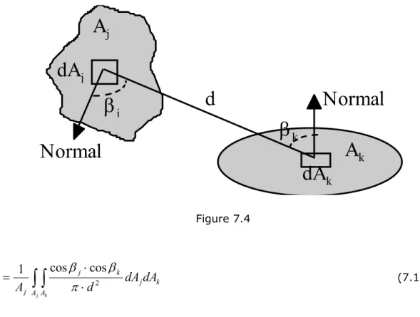
7.4 Calculation of view factors ... 65
7.4.1 View factors for basic configurations ... 67
7.4.2 Use of the addition rule ... 70
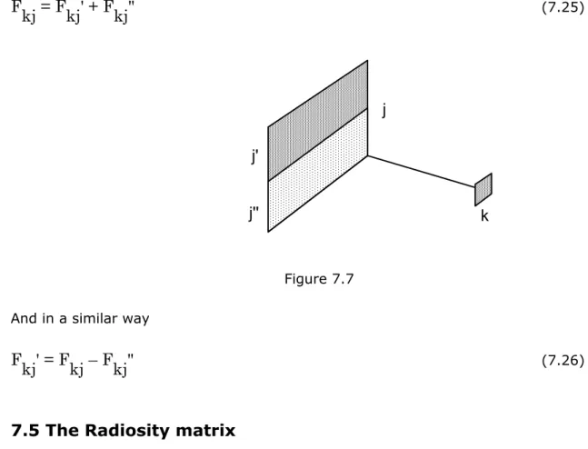
7.5 The Radiosity matrix ... 70
7.6 Combined radiation and convective heat transfer ... 72
8. SOLAR RADIATION ... 73
8.1 Solar radiation in building design ... 73
8.2 The elements of solar radiation ... 73
8.3 Calculation of the solar radiation towards an arbitrary surface ... 74
8.4 Solar radiation on a cloudy day ... 78
8.5 Heat balance on exterior surfaces ... 78
8.5.1Window heat balance ... 79
9. DUCT FLOW ... 85
9.1 Heat balance in a duct with air flow ... 85
9.2 The heat balance for a ventilated air gap ... 86
9.2 Non steady heat transfer in ducts with high thermal inertia ... 88
9.4 Hybrid systems for heating and cooling ... 92
10 LOW EXERGY DESIGN ... 96
10.1 General heat balance problems ... 96
10.2 The building components ... 96
10.3 The supply side ... 98
10.4 Heat balance for a building ... 99
11. APPENDIX I. DATA FOR CALCULATIONS ... 101
12. REFERENCES ... 103
LIST OF SYMBOLS
A Area m
2a Thermal diffusivity for a material m
2/s
a Solar asimut –
a Apsorptance for solar radiation –
A Complex matrix element –
Absorptance for long wave radiation –
B Complex matrix element m
2K /W
Volume expansion coefficient K
–1 horizontal angle –
B
0Specific permeability of the material m
2c Specific heat capacity, capacitivity J/kgK
C Thermal capacity J/K
C Complex matrix element W/m
2K
Point thermal transmittance of a thermal bridge W/K CCF Cloud cover factor – D Complex matrix element –
Declination from a plane through equator rad E Complex matrix element W/m
2K
E Energy J
Emissivity –
Heat flow rate J/s
F Complex matrix element W/m
2K F
abConfiguration factor or view factor from a to b –
The latitude of a location rad F Total window transmittance for solar radiation – F
1Partial window transmittance (Short-wave radiation) – F
2Partial window transmittance (Surface heat flow) – G Complex matrix element W/m
2K g Acceleration of gravity, 9.81 m/s
2Gr Grashof number –
h Coefficient of surface heat transfer W/m
2K H Complex matrix element W/m
2K
h solar altitude rad
H Height above a reference level, m
Dynamic viscosity of a fluid Ns/m
2I Solar radiation W/m
2i Angle of incidence rad
Temperature C
Heat production per unit volume W/ m
3J The total radiosity from an opaque surface W/m
2 Dynamic length coefficient rad
1/2/m
Thermal conductivity W/mK
Thermal conductance Alt: s W/K l Characteristic length m
l Length m
L Air flow m
3/s
fFriction coefficient. –
m Mass kg
M Total excitance of a real surface W/m
2M Cloudiness factor –
Form factor –
M° Total hemispheral excitance, black body W/m
2 Kinematic viscosity m
2/s
Nu Nusselt number –
p Static pressure, Pa
Pr Prandtl number –
Q Heat, energy J
q Density of heat flow rate W/m
2 Density kg/m
3R Thermal resistance m
2K/W
r ground reflectance –
R Gas constant, 8314.3 J/(kMol
.K)
Re Reynolds number –
Stefan Boltzmann constant = 5.67 10–
8W/m
2K
4.
T Temperature K
reflectance –
t Day number –
U Thermal transmittance by area W/m
2K
u Air velocity m/s
V Volume m
3v wall asimute –
x Length coordinate m
Pressure loss coefficient –
y Length coordinate m
Linear thermal transmittance of a thermal bridge W/mK
Indexes
a Ambient
c Convection (often includes conduction) d Diffuse
D Direct e Exterior equ Equivalent H Horizontal H Hydraulic i Inner, interior N Normal
r Radiation s Surface se Exterior surface si Inner surface V Vertical
TABLE
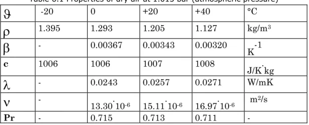
Table 6.1 Properties of dry air at 1.013 bar (atmospheric pressure) 49
Table A1 Thermophysical properties of materials 101
FIGURES
Figure 2.1 ... 16
Figure 2.2 ... 17
Figure 3.1 ... 18
Figure 3.2 ... 20
Figure 3.3 ... 22
Figure 3.4 ... 23
Figure 3.5 ... 24
Figure 3.6 ... 25
Figure 3.7 ... 27
Figure 4.1 ... 31
Figure 4.2 ... 32
Figure 4.3 ... 36
Figure 4.4 ... 38
Figure 5.1 ... 40
Figure 5.2 ... 41
Figure 6.1 ... 48
Figure 6.3 ... 51
Figure 6.4 ... 53
Figure 6.5 ... 54
Figure 6.6 ... 56
Figure 6.7 ... 57
Figure 7.1 ... 61
Figure 7.2 ... 64
Figure 7.3 ... 65
Figure 7.4 ... 66
Figure 7.5 ... 66
Figure 7.6 ... 67
Figure 7.7 ... 70
Figure 8.1 ... 74
Figure 8.2 ... 75
Figure 8.3 ... 76
Figure 8.4 ... 77
Figure 8.5 ... 79
Figure 8.6 ... 80
Figure 8.7 ... 83
Figure 9.1 ... 86
Figure 9.2 Ventilated air gap ... 86
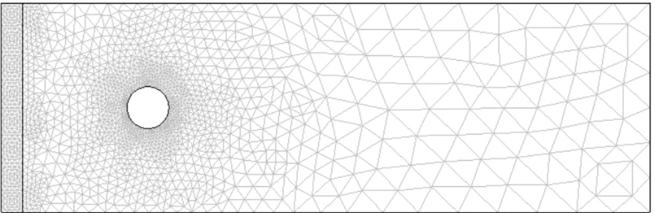
Figure 9.3 Finite element mesh for the problem. ... 89
Figure 9.4 The real part of the calculated emittances for the steady state solution for the steady state solution and the for first frequencies corresponding to periods of 1, ½, 1/3, and ¼ years ... 90
Figure 9.5 The imaginary part of the calculated emittances for the steady state solution for the steady state solution and the for first frequencies corresponding to periods of 1, ½, 1/3, and ¼ years ... 90
Figure 9.6 The magnitude of the calculated emittances for the steady state solution for the steady state solution and the for first frequencies corresponding to periods of 1, ½, 1/3, and ¼ years ... 91
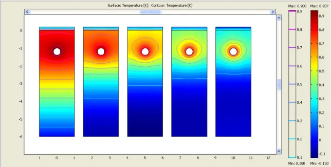
Figure 9.7 The annual variations in temperatures for a 60 m long duct coil with a diameter of 400 mm laid in a spiral at a depth 1000 mm with cc (center to center)
distance of 2000 mm with 200 mm EPS insulation on the top. ... 91
1 PREFACE
Around 40 % of the energy used in the world is used in buildings. Most of this energy is used to maintain an indoor environment that provides human comfort and functionality but also to create a suitable environment for industrial processes and storage of goods.
We provide daylight, electrical light, heating, cooling, fresh air, control the level of humidity etc. At the same time the fundamental thermodynamic principles apply. Our systems will always tend to change in the direction of maximum entropy. Conduction and convection of heat, diffusion and convection of vapor, oxygen and other gasses and the absorption of light are processes that will counteract our efforts to maintain a certain state off balance with the natural environment.
This book is about how we can minimize the entropy production in the processes involved in maintaining a defined indoor environment. Another way to put it is that we want to minimize the exergy loss in the system. By introducing the concept of exergy into our analysis we try to get a deeper insight into how the processes can be improved to bring the need for high quality auxiliary energy to a minimum. This means that we are not only looking at the amount of energy needed to maintain our environmental parameters but also the energy quality. We would therefore make big distinction between a house that needs annually 10000 kWh of electricity for space heating or a house that needs 10000 kWh of district heating water delivered at 80 OC and returned at 30 OC. In simpler terms it can be stated that we generally try to provide heating with minimum temperature difference between the heating or cooling medium and the indoor environment. This means that the heat transfer has to be distributed over larger surfaces and one way to achieve this is to integrate the heating or cooling processes into the building components such as floors, walls and ceilings. This however calls for a more advanced set of solutions compared to conventional systems.
The book is based on my lectures in building physics in my time as a professor at KTH [15] and also my research activities starting in the mid-seventies until today that have focused on solving heat transfer problems mostly involving thermal stability of buildings and the practical solutions for modelling construction integrated heat distribution systems for developing low temperature systems for heating and cooling and a more effective use of the thermal capacity [10]. A number of such applications more often developed within PhD and MSc work can be found in the references, [1; 21; 22; 29].
This book assumes that the reader has basic knowledge on conventional analysis of building heat transfer. The ambition here is to look deeper into the processes and provide means to model the processes in a more detailed manner, to provide tools for modeling integrated processes and to bring the analysis of the building as a system one step further to include the quality of energy as well the quantity of energy. The analysis will be limited to studying the processes in a steady or quasi steady state. Simulations of the operations of whole buildings and its systems in the time domain is beyond the scope of the text.
January 2013
Gudni A. Jóhannesson
2. BUILDING PHYSICS
Building physics is the science of climate protection in buildings and in built structures.
We build and heat houses to create a comfortable indoor climate, which can be maintained within specified limits, regardless of the variations in outdoor climate. To gain this we need structures that can withstand the external and internal forces of wind, snow and life loads but also to provide the structures with qualities such as thermal insulation, air and rain tightness, solar radiation control, sound insulation and biological protection.
Furthermore, our task is not only to provide for a good indoor environment, but also to provide for an environment within the building structures and for the building materials that does not enhance the decay of the structures due to corrosion, mould growth and rot, cracking due to thermal or humidity related stresses and so on. This even applies to constructions that are not parts of a climatic shield such as bridge and road constructions etc. where the decay and lost performance in many cases is more due to environmental factors than to the loads over time. Thus the construction of a built structure for optimum performance and durability has to be based on extensive knowledge on both structural mechanics and building physics.
2.1 What building physics is mainly about
When we describe the physical state within a building or a building structure we usually refer to the temperature, the air pressure and the moisture content. By moisture we mean water in different phases. The physical state can either be the result of our observations and calculations or give the initial and boundary conditions for further calculations. The combination of temperature and moisture content can for instance give us the risk estimate for fungi growth and rot in wooden construction parts and the distribution of temperatures in a rigid construction part can be used to estimate thermal stresses. We are also interested in how heat, air and moisture are transferred within our structures and systems. The potentials for these processes can be expressed as the physical parameters, the temperature, the air pressure and the moisture content respectively.
2.2 Examples of heat and mass transfer
A common example of the heat transfer process is the heat flow from the warm indoor environment through an insulated wall to the cold outdoor environment. This can involve heat conduction through parallel material layers as well as the treatment of two or three- dimensional material layers as well as the influence of air movements in the construction.
During wintertime the warm indoor air has lower density than the cold surrounding outdoor air. Thus by Archimedes law, the lightweight indoor air creates a force on the inside of the roof and the upper parts of the building relating to the weight difference between the outdoor and indoor air creating a pressure difference across the roof construction. The pressure difference in its turn will generate air flow through the roof through different leakage paths which may consist of air gaps, holes, cracks and porous materials.
2.3 Combined processes
Even if this book gives the transfer processes as separate chapters the processes we deal with in reality usually are combinations of these processes. As discussed above a temperature difference generates a pressure difference, which generates air movement, which in turn may affect the temperature difference. Since we are dealing with processes that can be non-linear, the complexity of the general solution of a problem has often been beyond what can be treated in normal engineering work and the problems have often been studied in an oversimplified way.
2.4 New mathematical tools make life easier
With the new mathematical tools available for personal computers such as the latest versions of Mathcad, Maple, Matlab and multiphysics finite element codes such as Comsol the application of building physics has come into a new and revolutionary era.
Figure 2.1
If the user knows the governing transfer equations, boundary conditions and construction and material parameters and links the transfer equations into balances that provide for the conservation of energy and mass, the solutions will be given by the computer. The
transfer equations can be non-continuous and the transfer parameters can be non-linear i.e. varying with the physical state such as the temperature or the moisture content.
2.5 Building physics and the environment
When addressing the environmental issue, important parameters are the performance and the durability of the construction.
Figure 2.2
One cubic meter of insulation in a well performing insulated construction may under its lifetime reduce the heating demand for the building with 5 cubic meters of oil compared to a poorly insulated construction. The main environmental issue is therefore not only the environmental qualities of the materials used, but also that the materials used will serve their purpose in an optimum way, regarding technical and economical as well as environmental factors. With increased durability and service life of the construction, the embedded environmental impact per year of use is reduced. Bad design of insulated constructions also creates favorable conditions for biological growth which may endanger indoor air quality and human health and in general have negative consequences for the indoor environment and comfort.
3. INTRODUCTION TO BUILDING HEAT TRANSFER
3.1 The basic elements of building heat transfer
There are numerous extensive textbooks on general heat transfer available, [4; 5; 7 20].
In this book the idea is to give a selection of the parts of general heat transfer that are frequently applied in building heat transfer to serve as basis for higher education and research and development within the field.
3.1.1 Temperatures
Figure 3.1
Temperatures are in this text either expressed as the thermodynamic temperature T, K, or the Celsius temperature
, °C. They are related as follows.
= T-273.15 (3.1)T =
+273.15 (3.2)Your thermodynamic body temperature is normally 310.15 K and can rise up to about 315 K when you get very ill.
3.1.2 Heat – a form of energy
For a certain amount of energy stored or released in the form of heat we use the quantity Q, J (joules). Before the unit for heat was calorie, which is the quantity of heat needed to heat one gram of water by one degree on the Celsius scale. One calorie is 4.184 J. In
0 °C
273.15 K
American literature the unit BTU (British thermal unit) is still used. One BTU is 1054.35026448 J, to be exact.
For the amount of heat produced or transferred per time unit we use the term heat-flow rate
, W = J/s. The unit J/s is also called watt.The following processes can release approximately equal amount of heat per time unit:
– Electrical radiator of 500 watts – Burning 0.05 liter of oil per hour – Burning 0.3 kg of wood per hour
– Solar radiation absorbed on a tilted surface of 0.5 m2 around noon on a clear day in June
– 4 persons working in a factory – 2 cows at rest.
3.1.3 Heat storage – heat capacity
If, for a body or a whole system, the temperature is raised by dT as a result of adding a small quantity of heat dQ then the heat capacity is defined as
C = dQ/dT J/K (3.3)
If the body is made of homogenous material the specific heat capacity c is defined as heat capacity divided by the mass m
c = C/m J/(kg.
K) (3.4)
or with known density
, kg/m3, and volume, V, m3 c = C/(V.
) J/(m3K) (3.5)Correspondingly the heat capacity for a given volume of material with specific heat capacity c is given by
C = V.
.c J/K (3.6)The amount of heat stored in a body or a system with heat capacity C, always has to be expressed in relation to some reference temperature T
ref to which the system is supposed to be cooled during the process of utilizing the stored heat.
The following systems can store approximately equal quantity of heat, or energy, which can be transformed to heat.
Figure 3.2
– 1 m3 water tank at 50 K above reference temperature
– 100 m2 concrete deck, 0.2 m thick at 5 K above reference temperature – 200 m3 of water stored at 10 m above reference level
– 70 ordinary car batteries – 5 liters of gasoline
3.1.4 Energy quality – exergy
The first law of thermodynamics tells us that energy can be transformed from one form to another but energy cannot be produced or consumed, [23]. This is in good accordance with what has been stated above. The second law of thermodynamics says that for all transformation processes for energy in a closed system the exergy content will be lower than in the original state. Therefore exergy can be lost contrary to energy. But what is exergy?
For a certain amount of energy in a given state, the ability to perform work is limited to only a certain fraction of the energy content. The exergy contained in this amount of energy is defined as the theoretical maximum amount of work that can be performed by transformations that bring the energy amount to the prevailing state of a reference environment. Electrical energy is approximately 100 % exergy while the ratio of exergy to energy or the energy quality of water at 80 °C is about 12 % for a reference state at 0
°C and the energy quality of energy at room temperature is then only 6%. The remaining part of the energy, which is not transformed into work, is in the transformation process fed to the environment at the environmental reference state or temperature and therefore its value for any use is lost. This part is called anergy.
The exergy per mass unit of material in a given state is expressed in terms of the differences in physical state between the actual state 1 and the reference state 2. The specific exergy, e12, J/kg is expressed in terms of the temperature, T, K, specific heat capacity cp, J/(kg K), height above reference level, z, m, velocity u in m/s, the pressure P in Pa, density in kg/m3 and the chemical exergy, CEX in J/kg, which includes all exo- or endothermic transformations such as chemical reactions and phase changes that takes place in the transformations between the two states:
1 2
2 2
2 1 2
12 1 2
1 2
1 2
(1 ) ( ) ( )
2
( )
T T p
T u u
e c T dT g z z
T p p
CEX
(3.7)
In many applications the influence of velocity and height can be neglected. For a stationary mass the exergy can be calculated from the data on enthalpy and entropy for the mass. For water and enthropy and enthalpy are found tabulated in a wide range of temperature and pressure. . A practical expression for the exergy then becomes as expressed by [4]:
12,spec 1 2 2( 1 2)
e h h T s s (3.8)
For a given volume of material with heat transfer to a colder environment the temperature and thereby the quality of the energy will be gradually lowered in the heat transfer process. The exergy content Ex12 for a given mass m, kg, with specific heat capacity cp, J/Kg.K, at a constant pressure, at rest and with no changes in chemical exergy can be found by integration as:
12 1 2 2 1
2
( ) ln
p
Ex c m T T T T T
(3.9)
3.1.5 Heat conduction
If we have two systems or bodies at different temperatures T
1 and T
2 which are in some way thermally connected, heat will flow from the warmer to the colder
= (T 1 – T 2)· W
(3.10)
(Big lambda), is the thermal conductance, W/K.In many problems we have a uniform two dimensional cross section over a longer distance L, m. An example is an insulated pipe or a duct. We define the linear thermal conductance as
= (T 1 – T 2) · · L, W
(3.11)
(Big psi) is the linear thermal conductance, W/KIf within a body of an isotropic material there exists a temperature gradient, grad T, the density of heat flow rate q can be calculated as
Figure 3.3
q = – · grad T, W/m
2 (3.12)This is often referred to as Fouriers law.
is the thermal conductivity of the material, W/mK.If T only depends on x, equ (3.12) becomes
, W/m
2The heat flow rate
through a surface with area A given by x = constant with a uniform temperature gradient then becomesx A T
(3.14)The thermal properties of a material are highly dependent on the structure and density of the material. What is referred to as the thermal conductivity of a porous material is often a combination of conduction, radiation exchange, convection and conduction in water in the pore structure. Examples of thermal properties of building materials are given in Appendix I.
3.2 Steady state calculations
In heat transfer calculations it is convenient to make a distinction between steady state and non-steady state heat transfer. Steady state means that the temperatures of the system do not vary with time. From the definition of the heat capacity
dQ = C dT
(3.15)x l m
T dx
dT T K
x
T
q
it is evident that in steady state heat is not being stored in or removed from any part of the system since this implies a change in temperature.
For a homogenous wall slab, with a temperature gradient in the direction normal to the surface, the consequence is, that if no heat is being stored at any point in the wall, the temperature gradient has to be constant. This also implies that the temperature is linearly distributed between the surfaces.
Figure 3.4
dT/dx = constant = (T 2- T 1)/ d
(3.16)The density of heat flow rate q, W/m2, can accordingly be expressed as
q (T2 T1)
d
d (T1 T2 ) , W/m
2(3.17)
This can also be written as
q (T 1 T 2 )
R W/m
2(
3.18)R d
m
2K/W
(3.19)is known as the thermal resistance of the wall slab.
T1
T2
d x
3.2.1 Steady state heat flow and temperature distribution in a multilayer wall with no internal heat sources
Figure 3.5
From the steady state condition it follows that the heat flow is constant through the construction
q1 = q 2 = q
3 = q 4 =.q
1 - Rn
n) 1 T - (Tn R2
3) 2 T (T R1
2) 1 T
q (T
...
(3.20)
or (T1-T
2)=q.R
1 (3.21)
(Tk-T
k+1)=q·R
k (3.22)
R
tot (R
k)
k1 n1
(3.23)q T
1 T
nR
tot (3.24)Assume that we have a known temperature T
1 on the left side of a construction and the heat flow q through the construction. The temperature difference across a layer k is given by
(Tk-T
k+1) = q·R
k (3.25)
Obviously the temperature in on the left boundary of a layer k can then be calculated as the sum of the temperature on the left side of the construction and the temperature differences across all layers on the left side of the boundary
11
1
1 1
1 k
j
k
j j j
k
T q R T q R
T
n ≥ k > 1 (3.26)
q T
1 T
nR
tot(3.27)
tot k
j j n
k
R
R T
T T
T
1
1 1
1
) (
(3.28)
3.2.2 Surface resistances
The heat transfer from a construction surface to the surroundings with a given temperature is taking place by radiation to surrounding surfaces and due to heat conduction and air movements close to the surface as will be treated in coming chapters.
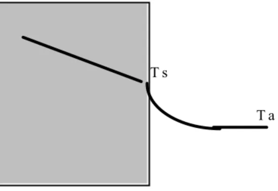
The coefficient of surface heat transfer hs, W/m2K, is defined as
Figure 3.6
T - T
h
q
s s a (3.29)
T s
T a
In practical applications, these complicated processes are often approximated by a fictive material layer between the surface, T
s, and an ambient temperature, T
a, which is often chosen as the air temperature.
R ) T - q (T
s a
s
(3.30) For simplified calculations in normal building applications these fictive resistances can be chosen on the inside towards a heated room with normal indoor climate
Rsi = 0.13 m2K/W (3.31)
and on the outside towards average external temperature and wind conditions
Rse = 0.04 m2K/W (3.32)
In reality however, the surface resistances vary greatly, due to miscellaneous factors, which will be further discussed in the lectures on radiation and convection in buildings.
3.2.3 Definition of the U-value
The thermal transmittance or U-value, W/m2K, for a construction is defined as the ratio between the density of heat flow rate q, W/m2, through the construction and the temperature difference between the ambient temperatures on both sides
U q (TiTe)
(3.33)
For a construction with n layers the U-value then becomes
U 1
R
si R
j R
sej1
n(3.34)
3.3 Two-dimensional heat conduction
We have so far learned that
1. The relation between the temperature gradient, thermal conductivity of a material and the heat flow rate known as Fouriers law.
2. The relation between a quantity of heat added to a given volume, the density and specific heat capacity of a given material and the resulting increase in temperature.
We are going to use these relations to establish a differential equality between the heat flow to an infinitesimal volume during an infinitesimal period of time and the increase in temperature. The aim is to establish a differential equation which describes the heat conduction process in a homogenous material
Assume a homogeneous material with material properties given as thermal conductivity
, density and specific heat capacity c.The temperature field within the material is given as
T=T(x,y,z,t) (3.35)
the heat flow rate at each point (x,y,z) is given as
q = - grad T (3.36)
The heat production per unit volume is given as
=
(x,y,z,t) (W/m3) (3.37)The heat production can for instance be due to a chemical reaction as in concrete being cured or due to absorbed solar radiation in a transparent insulation material. Let us look at a small element in Cartesian coordinates. Assume for simplicity that all variables are constant in the z direction that is
dT/dz = 0 and dz = 1 (3.38)
=
(x,y,t) (3.39)Figure 3.7
The regarded element has the dimensions dx and dy and one unit length in the z direction. Since the temperature gradient in the z direction equals zero the heat exchange between the element and the surrounding material goes through surfaces 1 to 4 and the areas of the sides of the elements are given by dx and dy respectively
y y+dy
x x+dx
c
During a small time step dt the quantity of heat added to the volume is
dQ = dt (
1 –
2 –
3 +
4 +
.dx.dy) (3.40)By using Fouriers law we can express the heat flow rates
1 = - dy (dT/dx)x(3.41)
2 = -dx (dT/dy)y+dy
(3.42)
3 = - dy (dT/dx)x+dx
(3.43)
4 = - dx (dT/dy)y
(3.44) Expansion by using the first two terms of Taylor
(dT/dx)x+dx = dT/dx +(d2T/dx2)x.dx (3.45) (dT/dy)y+dy= dT/dy +(d2T/dy2)y.dy (3.46) and substituting into equation (3.40) we get
dx dy
dy dx dT - dx )dx
T ( d dx dy dT dy )dy
T ( d dy dx dT dx dy dT - dt
dQ
22 22
. .
(3.45)
) dxdy
dx T (d dxdy dy )
T (d dxdy dt
dQ
22 22
. .(3.47)
From the definition of thermal capacity
dQ=
c.dx.dy.dT (3.48)
.c.dxdy.dT = dt (dx.dy +dx.dy)
) +
.dx.dy) (3.49)dx T ( d
22
dy ) T ( d 2
2
) c dx
T ( d dy )
T ( d c dt dT
2 2 2
2
(3.50)
The thermal diffusivity a for a material is defined as
a= /(
·c) m2/s (3.51)and if dt, dx and dy are made infinitesimally small
c ) ρ y
T x
a( T t
T
2 2 2 2
(3.52)which is the general equation for heat conduction or in more general mathematical terms
T/
t= a
T+ = a(
T+
/) (3.53)Equation (3.53) is valid in three dimensions as well.
4. HEAT CONDUCTION EQUATIONS – SIMPLIFICATIONS FOR NON-STEADY STATE SOLUTIONS
The conduction equation derived in chapter 3 in its general form is not easily solved analytically. The choice between numerical and analytical solutions is generally made on the basis of the relative cost effectiveness of the method chosen. The increasing availability of computers has lead into the direction of more frequent use of numerical methods. However new mathematical programs for personal computers now provide convenient tools for analytical or hybrid solutions.
4.1 Simplifications
By stating some limitations the equation can be simplified to a form where trivial analytical solutions can be found.
4.1.1 No heat production
Generation of heat within building materials is in most cases not relevant. The generation of heat can then be put equal to zero.
= 0
(4.1)The equation then becomes
T/t = a T
(4.2)4.1.2 No heat production with one dimensional heat flow
If we further assume that the temperatures are constant in the y and z directions it follows that
T/y =T/z = 0
(4.3)and the equation is reduced to
T/t = a .
2T/x
2(4.4)
4.2 Solution for a one dimensional slab with harmonic boundary temperatures
x=0 x
T 0
q 0
c
Figure 4.1
The following set of equations is based on [4]
A temperature variation that can be expressed as a sinus or cosinus function with time is called harmonic. By limiting the temperature variations at the boundaries to harmonic functions we can make use of their important properties that the derivative is equal to the function multiplied with a complex constant. Since heat conduction in building materials at normal temperature levels can be regarded as a linear process, all temperature variations within the system will be harmonic as well, but with different amplitude and phase lag. Since non-harmonic functions can be transformed to Fourier series, i.e. a sum of harmonic functions, problems with arbitrary boundary conditions can be solved in this way. A harmonic function always has the mean value zero. A rational technique is
– to solve the problems for the mean boundary conditions as a steady state problem – do the Fourier transform on the variations of the boundary conditions around the
mean value
– solve the response for the different frequency components as shown below – get the final result by superposition.
An important precondition for rational calculation work is that a harmonic function at a given frequency can be expressed ad a complex number relating the actual function to a basic oscillation.
The figure below shows how a harmonic oscillation can be expressed in the complex plane.
Figure 4.2
T =T
amp· ei (
t+
)
= (u+i v) · e i
t
(4.5) The time derivative of T then becomes
T/t = i T
(4.6)And the heat equation can be written as
i T = a(
2T/x
2)
(4.7)having a solution in the form
T= Csinh((1+i) x) + Dcosh((1+i) x)
(4.8)
2a
(4.9)This can be verified looking at the properties of the hyperbolic function and the complex i.
sinh(u) = (eu – e-u)/2 cosh(u) = (e u + e-u)/2
(4.10)12
u v
t
t 2
0
Tamp
2 i) (1 2 2
i 1
i
(4.11) The properties of the basic functions at x = 0
sinh(0)=0 cosh(0)=1
(4.12) together with a known boundary temperature at x = 0.
T=T(0)=T
0(4.13)
gives the unknown coefficient D
D=T
0(4.14)
If we now apply Fouriers law we get the equation for the heat flow
q(0)=(- dT/dx)
x=0=- C(1+i) cosh((1+i) . 0) + ... sinh(0)
(4.15) which gives C in terms of the heat flowC=(-q
0)/(
(1+i)
)
(4.16) and we can express the temperature at any location x in terms of the temperature and the heat flow at the surface.
T (x ) T
0cosh ((1 i )
.x ) q
0.sinh ((1 i ) x)
(1 i )
(4.17)An Important simplification is when we have a semi-infinite body with x=0 at the surface.
At an infinite distance from the surface the temperature variations at the surface have vanished, or
x then T(x) 0
(4.18)q
0 (1 i) T
0.cosh((1 i) x)
sinh((1 i) x
(4.19)x Then sinh(x) cosh(x) (see equ. 4.10)
(4.20)and we can now for the semi-infinite body establish a relation between temperature and heat flow at the surface.
q
0= (1+i) . T
0 (4.21)And by substitution of equ. (4.21) into equ (4.17) we get
T(x)=T
0{cosh((1+i) · x)-sinh((1+i) · x)}
(4.22)T(x)=T
0e -(1+i)
x
(4.23) Expression (4.23) can as an example, be used to estimate the amplitude of the annual temperature variation as a function of the depth from the surface. From equation (4.17) the heat flows at the boundaries of a finite material layer can be related to the boundary temperatures. This can be formalized as a matrix equation relating the temperatures and heat flows at the boundaries by a two by two complex matrix.
~0 0
~ 1 1
1 1
~1 1
~
q D C
B A q
(4.24)
A 1 cosh((1 i) 1d1)
(4.25)
B 1 sinh((1 i) 1d1)
1(1 i) 1
(4.26)
C 1 1(1 i) 1 sinh((1 i) 1d1)
(4.27)
D 1 cosh((1 i) 1d1)
(4.28)
4.2.1 Solution for a multilayer construction
A resulting matrix for a multilayer construction with n layers can then be calculated by a simple multiplication of the 2×2 matrices for the single layers. A matrix relation between heat flows and temperatures on both surfaces can in this way be established.
q~soso v~~
D ~ C
B A q~sisi
~
(4.29)
A B C D
A n Bn Cn Dn
A n 1 Bn 1 C n 1 Dn 1
.... A 1 B 1 C 1 D 1
(4.30)
Purely resistive layers such as surface layers and air gaps can represented by a matrix as well in order to calculate the heat flows at the ambient temperatures.
A k B k C k D k
1 R k
0 1
(4.31)
Equ (4.29) can be rearranged to give the heat flow variations as a function of the temperatures on both sides
so si so
si
H G
F E q
q
~
~
~
~
(4.32
) E=D/B F=C-DA/B G=1/B H=-A/B
(4.33)Equation (4.33) is most useful to study the dynamic behavior of multilayer constructions.
This is the basis for the work on an equivalent or so called active heat capacity in [10]
and later introduced as effective heat capacity in international standards. In [4] a solution for cylindrical geometries is also to be found and this has been corrected for minor errors and applied for study of borehole dynamics in [29]
4.3 Steady state heat flow – simplifications
By steady state heat flow we mean that the boundary conditions and generated heat are constant with time or
T/t = 0 (
4.34)The general equation for heat conduction is then reduced to
T + / = 0
(4.35)This equation is for instance useful when calculating the resulting temperatures in newly cast concrete slabs during the curing process.
4.3.1 Steady state one dimensional heat flow with heat generation If we further assume that the temperature is constant in the y and z directions we get
2T/x
2+ / = 0
(4.36)This equation can as an example be applied to a cooling fin or a relatively thin wall with thickness d, high thermal conductivity
and linear surface heat transfer coefficient hs = 1/Rs on both sides.2
x=0
d h
h
a
a s
s
x=L
Figure 4.3
The heat production can be expressed as the heat flow from the ambient temperature to the cooling fin per volume
(x) = 2·h
s· (T a- T(x))/d
(4.37)
2T(x)/x
2– 2·h
s· (T(x)-Ta)/(d· = 0
(4.38) By expressing (x) T(x) – T a and
hs.2
d.
(4.39)
and making the substitution, equ (4.38) becomes
2 /x
2–
2 = 0 (4.40)
having a solution in the form
Ce
xDe
x(4.41)
We assume that at x=0 the temperature is
from where it follows that
= C + D which gives C =
- D
(4.42)and, that the heat flow in the x direction at the farther end in x=L is equal to 0 which gives the other condition
(
x)L
CeL
DeL
(
0 D)eL
DeL 0(4.43)
De
bL De
bL
0e
bL(4.44)
Rearranging we get
bL bL
bL
e e
D e
0
(4.45)) (
) 1
(
00 L L
L L
L L
e e
e e
e
C e
(4.46)
L L
x L x
L
e e
e e e
e
0
(4.47)When
3
x L
this expression can with acceptable accuracy be given as
0e
x
(4.48)If we assume that the wall has a unit length in the direction perpendicular to the paper the heat flow from the base to the thin wall at x=0 can be expressed as
d(
x)0
(4.49) d 0 e L e L e L e L
(4.50)
d
0 tanh( L)
(4.51)In building physics equation (4.51) is useful to study the heat transfer along surface layers and attached wall or floor slabs toward a thermal bridge in an insulated wall. At values for
L above 2.0, tanh(
L)
approaches 1 and equation (4.51) approaches d
0(4.52)
This theory has been used as basis for the development of simplified equations for thermal bridges, [11], [21].
4.3.2 One dimensional steady state heat flow without heat sources
Since the temperatures are constant in time and in the y and z direction the general equation for heat conduction reduces to
d
2T(x)/dx
2= 0 (
4.53) Integrating on both sidesdT(x)/dx = konstant
(4.54)Figure 4.4 and we see that the trivial solution is
T(x) = T1+(x/d)(T2-T1)
(4.55) See chapter 3.
d x T 1
T 2
5. NUMERICAL METHODS
This chapter gives the basic knowledge for the reader to be able to model, from relatively simple principles, time dependent and two dimensional heat flow problems. For a deeper study into this subject see for instance [5]
5.1 The control element – two dimensional heat flow
We are going to us the same relations as in chapter 3 to establish a differential equality between the heat flow to an infinitesimal volume during an infinitesimal period of time and the increase in temperature. The aim is to establish a difference equation, which describes the heat conduction process in a homogenous material, on the border between two materials and on the surface of a material where we have convective and radiative heat transfer to an ambient temperature.
The temperature field within the material is given as
T=T(x,y,z,t)
(5.1) the heat flow rate at each point (x,y,z) is given asq = - grad T
(5.2)The heat production per unit volume is given as
= (x,y,z,t) (W/m
3)
(5.3)The heat production can as an example be due to a chemical reaction as in concrete being cured or due to absorbed solar radiation in a transparent insulation material.
We now look at a small element in Cartesian coordinates. Assume for simplicity that all variables are constant in the z direction that is
dT/dz = 0 (
5.4) = (x,y,t)
(5.5)Figure 5.1
The material field is divided into rectangular elements k,j that have the dimensions dxk and dyj and a unit length in the z direction. Each element can have material properties given as thermal conductivity,
, density, and specific heat capacity, c. Each element is represented by its temperature at a nodal point in the center of the element.Since the temperature gradient in the z direction equals zero the heat exchange between the element and the surrounding material goes through surfaces 1 to 4.
During a time step dt the quantity of heat added to the volume is
dQ = dt (
1+
2+
3+
4+ · dx· dy)
(5.6)Between each adjacent pair of nodal points we have a two layer construction with dimensions given by dx and dy. The heat flow between two adjacent nodal points can be calculated according to chapter 3.
x
dy
dy
dy
dx k-1 dx k dx k+1
j-1
j
j+1
k,j k+1,j
k,j+1 k-1,j
k,j-1 T
T
T T T
y
Figure 5.2
If all the heat flows are defined as directed towards the element k, j we get
1 =
k-1,k = (Tk-1 – Tk,j) (5.7)
2=
j-1,j= (T
j-1– T
k,j)
(5.8)
3=
k+1,k= (T
k+1– T
k,j)
(5.9)
4=
j+1,j= (T
j+1– T
k,j)
(5.10)We define the conductance s between adjacent elements as
k-1,k= s
k-1,k(T
k-1– T
k,j)
(5.11)
j-1,j= s
j-1,j(T
j-1– T
k,j)
(5.12)
k+1,k= s
k+1,k(T
k+1– T
k,j)
(5.13)
j+1,j= s
j+1,j(T
j+1– T
k,j)
(5.14)(5.15)
s
k-1,k=
s
j-1,j=
(5.16)
dy
k-1 dx
2 k
j
dx
2 T T
k-1 k
dx
kdy
j12
j1
dy
j2
j
dy
jdx
k12
k1
dx
k2
k
dx
kdy
j12
j1
dy
j2
j
dy
jdx
k12
k1
dx
k2
k