AND ECONOMIC ANALYSIS Fővám tér 8., 1093 Budapest, Hungary Phone: (+36-1) 482-5541, 482-5155 Fax: (+36-1) 482-5029 Email: erno.zalai@uni-corvinus.hu
W ORKING P APER
2003 / 5
T HE VON N EUMANN M ODEL AND THE E ARLY M ODELS OF
G ENERAL E QUILIBRIUM
Ernő Zalai
Budapest, 2003.
Ernő Zalai, BUESPA, Budapest1 1. Introduction
John von Neumann was a versatile scholar, whose path breaking ideas have enriched various disciplines. He has also made contributions of great importance to economics, although his only paper that was directly concerned with economics was his article on balanced economic growth, presented first at a Princeton seminar in 1932.2 We hasten to add that his influence on the later development of economics became equally important through his ground-breaking work on game theory. He was the first to prove the existence of equilib- rium for two-person zero-sum games in 1928, and their book (with Oskar Morgenstern) on game theory, published in 1944, was path-breaking in that field. Game theory, which studies the rules of rational human behaviour, is however an independent methodological discipline in itself and its domain is wider than economics.
Von Neumann’s model of general equilibrium can be linked to some common and critical points of departure of different competing schools. Von Neumann’s model was on the one hand a brilliant mathematical synthesis of the classical ideas concerned with the proportions required by economic equilibrium. It was on the other hand a forerunner of modern mathe- matical economics, which became fully developed only some decades later, under the influ- ence of neoclassical economics. Von Neumann generalized and employed for the first time Brouwer’s fixed-point theorem in the proof of existence of competitive equilibrium, and used an explicit and full duality approach and the linear activity description of technological choice.
Von Neumann’s model addressed very deep economic issues and it is no surprise that it can be fitted into most economic schools, into the at times Procrustean bed of neoclassical, Marxian or neo-Ricardian theoretical frameworks. And it has often been done so, after a few years of a surprisingly chilly reception of his model. (It suffices to refer here to the famous dispute between Solow and Kaldor at the 1958 Corfu conference, in which Kaldor strongly refuted the claim that the model of von Neumann was the “neo-classical school in a new dis- guise”. See Lutz and Hague, 1961, pp. 296-297).
If not for other reasons, but because of the aforementioned merits of the model, one may understand R. Weintraub’s enthusiasm when he went as far as stating “von Neumann’s paper is, in my view, the single most important article in mathematical economics” (Weintraub, 1983, p. 13). Weintraub’s judgement is however not shared universally by economists. At a 1974 conference in Warsaw Koopmans, while praising the many novel methodological
1 A slightly revised version of the paper will be published in Acta Oeconomica in 2004. The author wishes to acknow- ledge the valuable comments given by P.G. Hare, H. Kurz, J. Móczár, T. Révész, A. Simonovits and J. Varga on earlier versions of the paper.
2 Published in German in 1937, titled as “Über ein ökonomisches Gleichungssystem und eine Verallgemeinerung des Brouwerschen Fixpunktsatzes” (On an economic system of equations and a generalization of Brouwer’s fixpont theorem).
The title of the English translation became “A Model of General Equilibrium” and was published only in 1945.
aspects of the model, added “(t)he tremendous influence of von Neumann’s paper demonstra- tes that contributions of great importance can be made in a paper that is not very good eco- nomics” (Koopmans, 1974, p. 3, emphasis added). Samuelson, who also seemed to share Koopmans’ dry verdict, in his 1989 paper tried to downgrade the methodological importance of von Neumann’s model as well. Nevertheless, he had to acknowledge that: “He darted briefly into our domain and it has never been the same since” (Samuelson, 1989, p. 121).
The appearance of von Neumann’s model coincided with two important developments, which left lasting effects on the development of mathematical economics and explains partly its controversial reception too. One was the rise of quantitative economics3 as an independent sub-discipline in the early 1930s. Another and strongly related development was the gradual expansion of the axiomatic, a priori modelling approach that resulted in a shift from ‘ex ante’
to ‘ex post’ modelling, to “a philosophy of model-building which was borrowed from Hilbert’s metamathematics, to which von Neumann contributed substantially” (Punzo, 1989, p. 30). This change has gradually reached economics too, as Weintraub (1983, 1985) described very vividly. The number of mathematically trained and oriented economists has been steadily growing. They have brought into economics a radically changed perception of the subject matter and the methodology of mathematics (‘Bourbakism came to mathematical economics’, cf. Weintraub and Mirowski, 1994).
The adoption of the formal axiomatic approach and mathematical reasoning did accelerate the development of mathematical economics, but this progress incurred significant costs too.
The focus of research had swiftly shifted from the applied (concrete) to the pure (abstract), to
‘implicit theorising’ (Leontief). The requirements of logical consistency and mathematical elegance gained power over empirical relevance. Mathematics, “because of the lack of sufficiently secure experimental base” (Debreu, 1991), became increasingly a tool of logical calculus, instead of providing means for making quantitative empirical predictions. Beyond the traditional ideological and methodological schisms, the economics profession became further divided by language (verbal vs. mathematical) and methodology (analytical-formalist vs. historical-social) as well.
Marshall, one of the founders of modern economics, was among the first who warned against the extensive and unjustified use of mathematics in economics, because it “might lead us astray in pursuit of intellectual toys, imaginary problems” (Pigou, 1925, p. 84, quoted by Ekelund and Hébert, 1997). Von Neumann was also very much aware of the dangers in- volved, not only in sciences dealing with real phenomena, such as economics, but for the development of mathematics itself. “As a mathematical discipline travels far from its empi- rical source, or still more … if it is indirectly inspired by ideas coming from ‘reality’, … it becomes more and more purely astheticizing, more and more purely l’art pour l’art”
(Neumann, 1947, p. 234).
3 It has initially appeared under the name of econometrics, but later it became divided into three somewhat independent sub-disciplines: mathematical economics, operations research and econometrics. It is usually connected to the foundation of the Econometric Society (1930), and the journal of Econometrica (1933), although its roots can be traced back at least as far as to the book of Cournot (1838).
Although the model of von Neumann was in many ways a prototype of the a priori (ex ante) models in economics, he often cautioned against the misuse of such models. Morgen- stern (1976) recalls that von Neumann has repeatedly criticized economists for not using more appropriate mathematics and emphasized the need for more comprehensive mathema- tical tools than those borrowed from classical physics. It is perhaps not by accident that von Neumann did not continue his research on the abstract models of general equilibrium. Indeed, he did not just advocate the need for a new methodology, but, together with Morgenstern, set an excellent example for others to follow by their work on game theory, initiating a totally new discipline almost from scratch.
The paper is organised as follows. Section 2 reconstructs the way von Neumann set up his model. Section 3 contains notes on some salient aspects of the model and critically reviews some important attempts to generalise it. Some issues related to consumption, decompo- sability and uniqueness will be especially scrutinised. Although it is difficult to add much new to the vast literature, the author would like the reader to find some fresh ideas and new insights too in this appraisal nevertheless. The remaining sections are devoted to the most prominent models of general equilibrium that appeared before or roughly at the same time as von Neumann’s paper. The static and stationary models of Walras, Cassel, Schlesinger and Wald, and Leontief will be revisited and compared with von Neumann’s. The author hopes to demonstrate that none of them had any noticeable influence on von Neumann’s model, which is genuinely distinct, ideologically free and methodologically very fresh and forward-looking.
And that is all true despite the fact that the model can be viewed as a brilliant mathematical metaphor of some deep-rooted visions, pertaining to the core issues of commodity production.
2. The von Neumann model of economic equilibrium
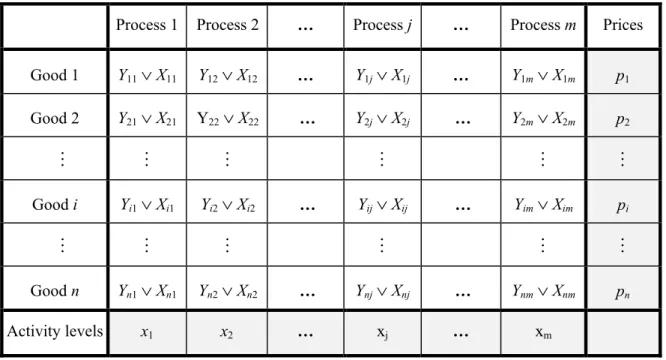
Table 1 illustrates the key components and the basic accounting framework of the model.
The rows (i = 1, 2,…, n) refer to economic goods, the columns (j = 1, 2,…, m) to economic processes. The table contains their lists and the amounts of the goods produced (Yij) and used (Xij) in the various processes in some period of time. The last column contains the unit prices of the goods and the last row the levels of the processes (activities). The latter refers to the intensities of operation of the processes.
Von Neumann considers an economy, in which production takes place in uniform, discrete periods of time, with exchange only at the turn of such intervals. By this assumption, the output of a given period can only be used in the next period. Because of the assumption of uniform production periods, he has to assume that “processes of longer duration (have) to be broken down into single processes of unit duration introducing if necessary intermediate products as additional goods”. He has also postulated that “capital goods are to be inserted on both sides of (the processes); wear and tear of capital goods is to be described by introducing different stages of wear as different goods, using a separate (process) for each of those”. In this way, he had actually turned fixed capital into circulating capital and assumed that capital circulation took uniformly one period time. He thus did not have to face the problems caused by the proper measurement of capital tied up in production.
Table 1. The basic accounting framework (goods, activities, inputs and outputs) in the von Neumann model
Process 1 Process 2 … Process j … Process m Prices
Good 1 Y11∨ X11 Y12∨ X12 … Y1j∨ X1j … Y1m∨ X1m p1 Good 2 Y21∨ X21 Y22∨ X22 … Y2j∨ X2j … Y2m∨ X2m p2
M M M M M M
Good i Yi1∨ Xi1 Yi2∨ Xi2 … Yij∨ Xij … Yim∨ Xim pi
M M M M M M
Good n Yn1∨ Xn1 Yn2∨ Xn2 … Ynj∨ Xnj … Ynm∨ Xnm pn
Activity levels x1 x2 … xj … xm
Von Neumann assumes that Xij, the amount of good i consumed in activity j, contains not only the direct material inputs of production but also the consumption of labour (and their households) engaged in it. For the sake of simplicity he also presumes that the consumption of the households consists only of necessities of life, and “all income in excess of necessities of life will be reinvested”, moreover, consumption patterns do not change over time and there is no technical progress. And a final assumption, “the natural factors of production, including labour, can be expanded in unlimited quantities”. The rate of growth depends thus on ‘man- made’ factors of production only, i.e., on the rate of accumulation of capital goods.
With these assumptions von Neumann defines an abstract, quasi-stationary economy, in which there is no reason for the proportions of the production and prices to change, once a state of equilibrium has been reached. The equilibrium of a quasi-stationary economy is a steady state, in which every physical quantity (the activity levels, the production and the use of various goods) changes by the same constant rate (λ). They increase, stagnate or decrease depending on the sign of λ.
In view of the rather stringent assumptions, von Neumann carefully avoided treating his model as a complete description of the working of a real economy, unlike some modern followers of general equilibrium theory. Quite to the contrary, he made clear that his model was a very abstract metaphor of a real economy, with the help of which one can shed light on some specific features of modern commodity production systems. He set out to analyze, first and foremost, the mutual dependence (‘remarkable dual symmetry’) of the rules guiding the selection of efficient (optimal) technologies on the one hand, and the determination of equilibrium prices (which make their use profitable) on the other, resulting from the circular nature of reproduction:
“In order to be able to discuss (the mentioned properties of the economic system) quite freely we shall idealise other elements of the situation … Most of these idealisations are irrelevant, but this question will not be discussed here” (ibid. p. 1).
He was aware that economics is as yet not a well developed scientific discipline and therefore the use of stringent abstractions is unavoidable. It is worth quoting him at length on this subject:
“It is frequently said that economics is not penetrable by rigorous scientific analysis, because one can not experiment freely. … Experimentation is a convenient tool, but large bodies of science have been developed without it. … What seems to be essentially difficult in econo- mics is the definition of categories. … it is always the conceptual area that the lack of exactness lies. … Now all science started like this, and economics, as a science, is only a few hundred years old. The natural sciences were more than a millennium old when the first really important progress was made. … methods in economic science are not worse than they were in other fields. But we will still require a great deal of research to develop the essential concepts – the really usable ideas.” (Neumann, 1955, in Bródy, Vámos, 1995, p. 639)
Let us now formulate, based on the above assumptions, the conditions of balanced supply and demand, using equations as his predecessors, following the classical “ex post” modelling approach:
Yi1 + Yi2 +…+ Yim = (1+λ)·(Xi1 + Xi2 +…+ Xim), i = 1, 2,…, n. (1) The equilibrium prices (pi, i = 1, 2,…, n) of such an economy must yield the same (π) rate of return (interest, as von Neumann called it) on capital in every activity used. The prices (as a matter of fact, only price ratios) can thus be defined by the following set of equations:
p1·Y1j + p2·Y2j +…+ pn·Ynj = (1+π)·(p1·X1j + p2·X2j +…+ pn·Xnj), j = 1, 2,…, m. (2) By dividing each equation by the level of the corresponding activity (xj) and assuming constant output (bij = Yij/xj) and input (aij = Xij/xj) coefficients (constant returns to scale), the equilibrium conditions can be rewritten into the following symmetric, dual forms:
bi1·x1 + bi2·x2 +…+ bim·xm = (1+λ)·(ai1·x1 + ai2·x2 +…+ aim·xm), i = 1, 2,…, n, (3) p1·b1j + p2·b2j + …+ pn·bnj = (1+π)·(p1·a1j + p2·a2j +…+ pn·anj), j = 1, 2,…, m. (4) As far as the economic content is concerned, there is nothing novel in the above descrip- tion of the conditions of equilibrium of an economy, its origins can clearly be traced back to the classical economists. Champernowne (1945) first asserted the classical origin of the model in his paper accompanying the English publication of von Neumann’s paper. A typical example of a similar quasi-stationary economic model is Marx’s scheme of simple and exten- ded reproduction, which in turn was inspired by the work of Quesnay. Sraffa (1960) has also used a similar model to analyse some features of long-term equilibrium prices. He has defined a “self-reproducing standard system”, in which production expands at an equi- proportional rate of growth, but that was not meant to be a model of actual production. (See
Kurz and Salvadori, 2001 for a comparison of the models of Sraffa and von Neumann and also for further references.)
This fact may explain the puzzling remark of von Neumann: “(i)t is obvious to what kind of theoretical models the above assumptions correspond“ (ibid. p. 2).4 What was novel in von Neumann’s approach was the precise mathematical reformulation of the classical concept for the case of joint production and choice of techniques, and the proof of existence of an equilibrium solution. Namely, unlike in other models of general equilibrium of his time, von Neumann took joint production (activities may produce several goods together) and techno- logical choice (the same commodity may be produced by several activities) explicitly into account in his model.
The above circumstances imply that the equation system (3) and (4) will be irregular (they will as a rule have much more variables than equations) and therefore the traditional method of counting equations can not be used. One can not assume, in general, that there exists a structure of production (x) for which goods are produced (Bx) and used (Ax) in the same proportions. Nor can one expect, in general, to find a price system for which the ratios of revenues (pB) and costs (pA) will be the same for each process. The systems of equation (3) and (4) may thus not have solutions at all. But even if they do, some variables may assume negative values, which would normally violate their economic content. To be more precise, one can not accept negative values for the activity levels or the prices if one assumes the irreversibility of the activities and free disposal. Indeed, von Neumann did implicitly adopt these assumptions by restricting the values of the activity levels and prices to be non- negative.
In order to solve the problem, von Neumann relaxed the equilibrium conditions. On the one hand, he introduced the possibility of excess supply of some goods and on the other hand, extra costs for some processes. In order to stay in line with the rule of supply and demand, von Neumann had to complement the above assumptions with two rules. Namely, any commodity in excess supply will be a free good and hence its price zero (the Rule of Free Goods), and the activities that do not yield the maximum rate of return will not be used in equilibrium (the Rule of Idle Activities).
Therefore, equilibrium conditions should be formulated as a complementarity problem and use the following system instead of equations (3) and (4):
∑j bij·xj ≥ (1+λ)·∑j aij·xj, i = 1, 2,…, n. (5a) pi·∑j bij·xj = (1+λ)·pi·∑j aij·xj, i = 1, 2,…, n, (5c)
∑i pi·bij ≤ (1+π)·∑i pi·aij, j = 1, 2,…, m. (6a)
xj·∑i pi·bij = (1+π)·xj·∑i pi·aij, j = 1, 2,…, m, (6c)
4 Von Neumann did not reveal the origins of his model. On the alternative interpretations of the von Neumann model see Kurz and Salvadori (1995, esp. pp. 407-414). We will also come back to this issue at the end of this paper.
Von Neumann was not the first to use complementary slackness conditions, which has become a standard tool in equilibrium models. In a different context Zeuthen (1933) and Schlesinger (1935) had also suggested the use of the Rule of Free Goods in order to avoid the negative prices in the Cassel model. But Von Neumann was the first to formulate duality and complementary slackness conditions in a symmetric, full-fledged manner.
As can be seen, the equilibrium conditions determine only the relative sizes (proportions) of the variables xj and pi. If some values of x and p satisfy the above system, then s·xj and v·pi
will also satisfy it, as long as s and v are positive scalars. The trivial solutions (no production at all, or nothing but free goods) have no economic relevance, so they can be ruled out at the outset. One can thus set the activity and price levels in any meaningful way. Von Neumann did it by setting their sums equal to one (∑j xj = ∑i pi = 1), that is, restricting their domain to the so-called standard (unit) simplex.
Observe that by multiplying both sides of inequalities (5a) and (6a) with the corres- ponding (complementing) pi and xj variables, respectively and taking their sum, one can derive the following series of inequalities:
(1+λ)·∑ij pi·aij·xj ≤ ∑ij pi·bij·xj ≤ (1+π)·∑ij pi·aij·xj. (7) There are two important conclusions that follow from the above inequalities. First, if the value of total output (∑ij pi·bij·xj) is positive, as required from any meaningful solution, then λ
= π, i.e. the equilibrium rate of growth and interest (return on capital) will be equal. Second, if in turn λ = π, then the complementary slackness conditions will be automatically met by the solutions of (5a) and (6a). Von Neumann postulated that aij, bij ≥ 0 and aij + bij > 0 for all i and j, that is, each commodity takes part in every activity either as input and/or output.
The above assumption guarantees that the value of total output will be positive in the case of any feasible (primal) solution and therefore the equilibrium rates of growth and interest will be equal and uniquely determined by the coefficients of the model. The same conditions imply also, as indicated above, the fulfilment of the complementary slackness conditions.
One can thus leave equation (5c) and (6c) out of the final form of the model and simplify it further by introducing a common factor of growth and interest (α = 1 + λ = 1 + π).
x, p ≥ 0, α > 0, (8a) 1x = p1 = 1, (8b)
Bx ≥ αAx, (8c)
pB ≤ αpA, (8d)
where (for shorthand we switched to matrix-vector notation) x = (xj), p = (pi), B = (bij), A = (aij) and 1 is a (summation) vector, the elements of which are all equal to 1. Von Neumann provided a rigorous proof showing the existence of a solution of the above system.
3. Some notes on the properties and generalizations of the von Neumann model
3.1. The uniqueness of the equilibrium in terms of the rate of growth and interest was crucial for von Neumann for at least two reasons. First, it made the duality of the two (quantity and value) sides of the model complete. The common equilibrium rate is the highest possible uniform rate of growth, on the one hand, and the smallest possible equilibrium rate of interest, on the other. In other words
λ* = α – 1 = max { λ : ∃ x ≥ 0, 1x = 1, Bx ≥ (1+λ)Ax }, (9a) π* = α – 1 = min { π : ∃ p ≥ 0, p1 = 1, pB ≤ (1+π)pA }. (9b) Second, this equality established the crucial mathematical link between the existence of equilibrium in the model of balanced growth and that of the two-person, zero sum games.
Von Neumann used the same minimax (saddle point) approach in both cases, based on the generalization of Brouwer’s fixed-point theorem.5
3.2. The equilibrium conditions in the growth model are, as von Neumann pointed out, the necessary conditions for a minimax solution (saddle point) of the following function:
F(x, p) = F(x1, x2… xm ; p1, p2 ,…, pn) = ∑ij pi·bij·xj / ∑ij pi·aij·xj, (10) where the denominator, the total value of the inputs, is assumed to be positive. Function F can be called the profit function, since its value at (x, p) determines the profit factor.
It is easy to show that (α*, x*, p*) is an equilibrium solution of the von Neumann model if and only if F(x*, p) reaches its minimum in p at p*, and F(x, p*) reaches its maximum in x at x*, where the value of F(x*, p*) is equal to α*, that is,
F(x, p*) ≤ F(x*, p*) ≤ F(x*, p). (11) 3.3. Von Neumann has called attention to an interesting formal analogy that exists between economic phenomena and thermodynamics. Namely, the role of the profit function
“appears to be similar to that of thermodynamic potentials”, and he conjectured that “the similarity will persist in its full phenomenological generality (independently from our restrictive idealisations)” (ibid. p. 1).
Thermodynamics and physics, in general, have significantly influenced the development of the methodology of economics. The founders of modern neoclassical analysis, Hicks (1939) and Samuelson (1947) borrowed, for example, the basic tools of their mathematical analysis from classical thermodynamics. Georgescu-Roegen (1971) devoted a whole book to illustrate similarities between economics and thermodynamics. More recently Bródy (1989) has revisited von Neumann’s conjecture and offered a potential explanation of its deeper meaning (see also Bródy, Martinás and Sajó, 1985, and Martinás, 2000).
5 Kakutani (1941) had provided later a more general theorem with much shorter proof that became the standard reference in the existence proofs of general equilibrium. As a matter of interest, Kakutani did not know von Neumann’s theorem when he prepared the first draft of his paper. He consulted nevertheless often with von Neumann as he was finalizing his paper for publication at Princeton (cf. Weintraub, 1983).
3.4. The uniqueness of the equilibrium rate of growth is of special interest because it means that it is the maximal rate of expansion allowed by the input-output coefficients. The unique path of steady state growth, called the von Neumann-path, exhibits an interesting property that was first pointed out by Dorfman, Samuelson and Solow (1959) and called aptly a turnpike (express highway) property. Several turnpike theorems have followed. They prove in essence that optimal growth paths, even if they start and terminate outside of the von Neu- mann-path, will run near to or on the Neumann-path most of the time, provided that the time horizon is long enough (see the review article of Koopmans, 1964, for references).
3.5. The assumption aij + bij > 0 guaranteed for von Neumann the existence and unique- ness of the common equilibrium rate of growth and interest. It is however a rather strong assumption that can not be defended on economic grounds. Kemeny, Morgenstern and Thompson (1956) have replaced it by much weaker postulates. At the same time they have simplified the existence proof without invoking a fixed-point theorem. The KMT conditions are as follows:
∑j bij > 0 for all i and ∑i aij > 0 for all j, (12) which state that each good is reproducible and that each process requires (directly) at least one product as input (either in production or in consumption).
Both postulates are quite natural assumptions. Von Neumann himself, as a matter of fact, adopted the first one, when he excluded the natural factors of production from his model. One needs the second one for exactly the same reason, to ensure that the rates of growth and interest remain finite despite the absence of exogenous resource constraints. (Incidentally, allowing for not only direct but indirect requirements too, one can further relax this assump- tion.) The above assumptions, however, do not guarantee that the total value of production will be positive (and the rates of growth and interest equal). As a consequence of this modi- fication, the positivity of the value of total output (∑ij pi·bij·xj > 0) had to be added to the equilibrium conditions, as a special requirement, in order to make the solutions economically meaningful and also to secure the equality of the two factors. We will refer to the resulting variant of the von Neumann model as the KMT model.
The same authors have also shown that under the revised conditions the equilibrium factor of growth and interest is no longer necessarily unique, that the number of possible values of factors is finite and can not exceed the minimum of the number of activities and the number of goods. Multiple solutions can exist if the model-economy is decomposable, meaning that some groups of activities can be operated without using goods that can be produced only by activities not belonging to that group.
3.6. The above uniqueness, as pointed out earlier, was crucial for von Neumann. He made that point clear as he commented on his assumption that aij + bij > 0: “it must be imposed in order to assure uniqueness of α, β (1+λ and 1+π in our notation) as otherwise W (the system) might break up into disconnected parts” (ibid. p. 3). This quote reveals also that he knew exactly that with his assumption he actually ensured the indecomposability of the economy.
Gale (1960) has therefore suggested relaxing von Neumann’s original assumption by simply postulating that all goods must be produced in any solution that fulfils the balance conditions
given by (5a). This is however the consequence rather than the proper definition of the in- decomposability of an economic system given by constant input and output coefficients.
Móczár (1995) provided a proper structural characterization of (in)decomposability, in terms of the input and output coefficient matrices of von Neumann.
A wide range of literature has been devoted to the consequences of decomposability in models of the von Neumann type. The mathematical properties of multiple solutions have been fully explored by several authors. The comprehensive characterizations given by Mori- shima (1971) and Bromek (1974a) deserve special attention. From a mathematical point of view the investigations are interesting, but the economic relevance of multiple equilibrium solutions, in terms of the rate of growth and interest, is in our opinion, to say the least, doubtful (we will come back to this issue later).
3.7. The only point that brought von Neumann closer to the neoclassical rather than the classical terminology is his usage of the term of interest instead of profit. He viewed profit, like most neoclassical economists, as an excess income above normal costs (including interest on capital), which the classical economists called ‘extra-profit’. This can be distilled from the passage in which von Neumann comments on the conditions of equilibrium: “in equilibrium no profit can be made on any process … else prices or the rate of interest would rise – it is clear how this abstraction is to be understood” (ibid. p. 3). This puzzling remark, typical of von Neumann, suggests that he must have assumed that in an economy “without monetary complications” the equilibrium rate of interest would be equal to the uniform rate of surplus or ‘profit’, using the latter term in its classical meaning.
Following von Neumann’s instruction, consumption can be explicitly introduced in the model6 by decomposing the inputs A = (aij) into uses in production R = (rij) and in consump- tion (cij), where aij = rij + cij. The cost of necessary consumption (wj = ∑i pi·cij) can be inter- preted as the unit wage cost because the cost of consumption enters the definition of prices in its place (material cost + cost of consumption + plus interest). What else could it represent anyway? Classical economists have also frequently used this simplifying solution, assuming that workers spend all their income on consumption. With this in mind, one can rightly replace interest with the classical notion of profit, whereby the equilibrium prices become the well-known prices of production, used by classical economists.
3.8. Morishima (1964) related consumption to the amount of labour used. He defined the consumption coefficients as cij = ci·mj, where ci is the amount of good i required for the reproduction of one hour labour and mj is the number of hours employed in activity j, operated at unit level of intensity. With matrix notation: C = c◦m, where symbol ‘a◦b’
denotes the outer product of vectors a and b. The hourly wage rate is thus w = pc = ∑i pi·ci, the total number of hours employed in the economy as a whole is L = mx = ∑j mj·xj and the total wage bill w·L = (pc)(mx) = p(c◦m)x = ∑ij pi·cij·xj. The equilibrium conditions in Mori- shima’s explication (concretion) of the von Neumann model take thus the following form:
x, p ≥ 0, α > 0, (13a)
6 See the review article of Bauer (1974) on the various possibilities offered in the literature.
1x = p1 = 1, (13b)
Bx ≥ α(R + c◦m)x, (13c)
pB ≤ αp(R + c◦m), (13d)
pBx > 0. (13e)
Such a generalization of the von Neumann model (by making its specification more con- crete) is perfectly legitimate, as long as one assumes that labour power is homogeneous and indispensable. This latter assumption means that reproduction can not take place at any positive level without using labour power. It can be postulated as follows: ∑j mj·xj > 0, for all xj ≥ 0 such that there exists α > 0, at which conditions (5a) are fulfilled in such a way that at least one good is produced.
It has been shown that for certain magnitudes of exogenously given consumption coef- ficients the KMT model may not have such a solution, in which the price of some ‘necessities of life’, that is the wage rate is positive. It has also been shown that some or all consumption coefficients could be increased in such cases without decreasing the rate of interest or growth.
What is perhaps even more important, Bromek (1974b) has shown that the common equilibrium rate of growth and interest must be the highest possible rate of expansion, whenever a positive wage can be associated with it.
3.9. This last observation is crucial and must hold for more general models too, if wages are defined as the cost of a given basket of wage goods. In such an interpretation and the corresponding extensions of the von Neumann model, one can thus re-establish von Neumann’s assertion that the equilibrium rates of growth and interest are equal and uniquely determined. One can in fact do it using a requirement that is somewhat weaker and more plausible than indecomposability. One simply augments the definition of equilibrium with requiring the positivity of the total value of consumption, ∑ij pi·cij·xj > 0 instead of the total value of production, ∑ij pi·bij·xj > 0 as Kemeny, Morgenstern and Thompson did. Note that this latter constraint of ours implies the KMT one, which is not necessarily the case the other way around, as noted above.
Any economist should ab ovo exclude solutions in which the value of consumption is nil.
In a model of long-term economic equilibrium, in which the consumption coefficients are given exogenously, in fact arbitrarily, one can not justify such a situation on sound economic grounds. Such a situation could not be sustained for any period of time. They are mathe- matical artefacts, totally irrelevant from the point of view of an economist. Von Neumann was thus completely right in our view to postulate that the common equilibrium rate of growth and interest is unique and maximal, although he failed to provide a convincing argu- ment for that. There is, however, one problem with that assumption. Namely, there is no easy way to guarantee that the equilibrium solution will be a saddle-point. This may disappoint some followers of von Neumann.
3.10. Let us now introduce a scalar variable to measure the level of (necessary) consump- tion and denote it by γ. The simplest way to let the level of consumption vary is to treat its structure constant. In such a case the cij (per activity level) consumption coefficients can be
determined as cij = γ·sij, where the sij coefficients are appropriately chosen structural cons- tants, and γ is variable, the level of which is set either exogenously or endogenously.
One could of course introduce more elaborate demand functions too. That would only make the model and the analysis technically more complicated, but hardly change the results.
For, one should be able to demonstrate a real trade-off between γ and α, i.e., to show that one is a strictly decreasing function of the other. Any meaningful demand system should fulfil this requirement. From the setup of the model it follows that γ represents both the level of consumption and that of the real wage, in the same way indeed as α stands for both the factor of growth and profit. The trade-off curve defined by the values of γ and α gives the (optimal) consumption-investment as well as the wage-profit frontier, as they are called in the neoclas- sical theory of growth.
The classical concept of wage-profit correspondence was reintroduced by Hicks (1939), as the factor-price frontier. Bruno (1969) proved and called attention to the duality (coinci- dence) of the wage-profit and the consumption-investment frontier in the neoclassical model of optimal growth. This was not the case in the KMT model because of the possibility of multiple equilibrium solutions. Morishima (1971) therefore reinterpreted their concepts and their duality for the von Neumann model. He redefined them as the maximal consumption- investment (primal) and the minimal wage-profit (dual) frontier, using definition (9a) and (9b) with a varying level of consumption. The two frontiers will as a rule differ in decom- posable economies. Morishima has in fact defined several (subordinate) frontiers, each corresponding to one of the equilibrium rates of growth (profit) feasible at the given level of consumption (real wage).
Bromek (1974b) on the other hand has proposed to re-establish the coincidence (the strict duality) of the two frontiers, by requiring the wage level to be positive in equilibrium, as we did before. Burmeister and Kuga (1970) suggested an almost identical solution in a somewhat more general intertemporal model allowing for joint production. Bromek has shown that γ is a strictly decreasing function of α, but it may be discontinuous at some (singular) points, if the system is decomposable. The domain of the inverse function, the consumption-investment frontier, will thus be disconnected at the corresponding values.
3.11. Let us confine the range of equilibrium solutions in Morishima’s explication of the von Neumann model by requiring the value of consumption (the wage rate) to be positive (pc
> 0). We must assume of course, as indicated above, that labour is indispensable (which guarantees that mx > 0 in any feasible solution). From the analysis of Morishima and Bromek it follows that the conditions of the equilibrium can be rewritten as follows:
x, p ≥ 0, α > 0, (14a) mx = ps = 1, (14b)
Bx ≥ α(Rx + γs), (14c)
pB ≤ α(pR + γm), (14d)
where γ is here the level of per hour consumption and the s = (si) coefficients the amounts consumed at unit level of γ. The level of γ is assumed to be given exogenously here, as in the case of the original von Neumann model.
All we have done was to set the levels of the variables differently, using the equations given in (14b). They together imply that the total value of consumption will be positive, as required for meaningful solutions, so there is no need to add them. Notice that for the same reason
(R + γs◦m)x = Rx + γs, and p(R + γs◦m) = pR + γm, (15) and this why we could replace inequalities (8c) and (8d), homogeneous in variables x and p, respectively, by their inhomogeneous counterparts.
System (14) provides a complete characterization of equilibrium in the extended von Neumann model, with homogenous labour and a parametrically changing level of consump- tion. It is equivalent to system (13), the conditions of Morishima’s model, except for the last one, which was replaced by pCx > 0 or p(s◦m)x > 0 in our case. This characterization of the equilibrium is interesting for several reasons. First, it introduces properly the real wage (w = γ) into the model by choosing the unit consumption bundle as numeraire (pc = 1). Second, this generalised form proved to be useful in comparing the analysis of von Neumann and Sraffa (see Kurz and Salvadori, 1995 for more details on this issue). But most of all, it allows one to change the exogenous-endogenous role of the growth (profit) factor and the level of consumption (real wage). One could do that both for technical advantages and in order to change the underlying economic hypothesis.
In the original model of von Neumann the level of consumption was determined exoge- nously. He did not refer to any mechanism that establishes its level and structure. He might have borrowed the concept of necessary consumption from classical economics. Once the level of necessary consumption is given, this determines the rate of profit and growth. But one could easily turn the causal relationship around: take the rate of growth as given exogenously and let the level of consumption become endogenous instead. One can, for in- stance, assume a steadily growing population and constant per capita consumption needs.
That will determine the necessary rate of growth, like in some neoclassical models of economic growth. (Cassel, as we will see shortly, assumed that all natural factors grew at the same constant rate.)
But, as long as the equilibrium rate of growth and profit is unique, there is a one-to-one correspondence between α and γ, that is between the feasible values of the growth factor and the level of consumption. From a purely mathematical point of view therefore it does not matter which is determined first. Once one of them is given, the level of the other is deter- mined too. In the analysis of the consumption-investment or the wage-profit function it proves to be useful to change the mathematical role of the two potential variables. For, as was pointed out, certain levels of consumption may not be associated with an equilibrium rate of growth. But this is not the case the other way around.
It easy to show (see Bromek, 1974b or Zalai, 2002) that the domain of the feasible equilibrium factors of growth (profit) is a connected set, H = (0; Λ), which is determined as
H = {α > 0: ∃ x ≥ 0, [(1/α)B − R]x ≥ s}, (16) where Λ is, under natural assumptions (i.e., constant capital is indispensable) a finite number and H may be closed from above, thus, H = (0; Λ].
It can also be shown that treating α as parameter (exogenous variable) and γ as (endo- genous) variable, the equilibrium of the generalised von Neumann model, system (14), can be found by solving the following (primal-dual) pair of parametric (α) linear programming prob- lems:
Primal problem Dual problem
y ≥ 0, x ≥ 0 w ≥ 0, p ≥ 0
[(1/α)B − R]x ≥ ys p[(1/α)B − R] ≤ wm (17)
mx ≤ 1 ps ≥ 1
y → max! w → min!
One can easily see the mathematical equivalence of the solutions of the two systems, by taking γ = y = w. This reformulation of the problem allows one to gain further interesting results by using the theorems and techniques of linear programming, with which economists are usually more familiar than with topology or convex analysis.
3.12. It is apparent that the equality of the equilibrium rate of growth and interest (profit) in the von Neumann model is a direct consequence of his assumption that all income in excess of necessary consumption is reinvested. It is also easy to show that the rates of growth and profit will as a rule differ if one introduces luxury consumption as well into the model.
Let us denote the coefficients of luxury consumption by fij. If we add them to the model, the coefficients determining total use (dij = aij + fij) and those defining the cost of production (aij) will no longer be the same. The basic inequalities of equilibrium in this extended model will be as follows:
∑j bij·xj ≥ (1+λ)·∑j (aij + fij)·xj , (5b)
∑i pi·bij ≤ (1+π)·∑i pi·aij . (6a) Clearly, the introduction of luxury consumption does not affect the definition of the profit rate and the prices. It can immediately be seen also that the above generalization of the von Neumann model abolishes its elegant (symmetric) duality.7 In the above extension of the von Neumann model the rate of profit sets an upper limit for the potential growth rate (λ ≤ π).
Under some normal conditions, the growth rate will decrease as the level (some or all coef- ficients) of luxury consumption increases. It can in fact increase to a level at which there will be no growth at all (λ = 0, the case of simple reproduction), whereas the rate of profit remains positive. This is again in perfect harmony with the classical analysis of the capitalist mode of reproduction.
7 See Morishima (1964) and ≡o∇ and ≡o∇ (1974) for more on this or similar asymmetric extensions of the von Neumann model.
4. The Walras–Cassel-model and its Schlesinger–Wald variant8
Let us turn our attention now to other salient models of general economic equilibrium that appeared prior to or concurrently with von Neumann’s model. The concept of economic equilibrium goes back at least to the classical economists who found a convincing analogy between the laws of nature and competitive markets (the famous “invisible hand” of Adam Smith). Both sets of laws seemed to be capable of securing long-term harmony, stability and efficiency. This ideal state is behind the concept of general economic equilibrium, and not just the law of supply and demand. The classical economists did not put that vision or parable into formal models. Even Cournot (1838), whom many consider as the first proper mathe- matical economist, saw the formulation of such model as easy, but completely useless for any practical purposes (because of a lack of data, computational methods and facilities).
Walras (1874) was the first who put aside such practical concerns and, in the spirit of pure science, ‘invented’ the first models of general equilibrium. In this sense, he is rightly considered to be the father of general equilibrium models. In the various editions of his famous book Walras presented a series of general equilibrium models of decreasing level of abstraction (pure exchange economy, production economy without and with capital goods). It is interesting to note that Marx, a contemporary to Walras, was the other economist who, in the words of the Nobel-laureate Arrow (1974), has got much closer to the modern theory and models of general equilibrium than any of his predecessors. He meant Marx’s two-sector schemes of reproduction and equilibrium prices.
Despite the priority of Walras, we will start our review with a model of Cassel, a Swedish economist. His formal (static) model can be seen as a simplified version of that of Walras (it is often referred to as the Walras–Cassel model). Cassel’s influence on later developments became more crucial than that of Walras. His model had attracted the attention of one of the famous Viennese circles of scholars in the 1920s. They were interested in the formal analysis of some concepts of the Austrian neoclassical school of economics. The problem at the focus of their attention was the so-called principle of imputation (Zurechnung).
Carl Menger (1871) divided the economic goods into the groups of final products and factors of production (of various orders). The equilibrium prices of the final products, in his view, are directly established by the consumers’ preferences, which in turn determine, via imputation, the prices of the factors of production (distributing the revenue among their suppliers). Once we know the prices (pi) and the input requirements (dki) of the products, the prices of the factors of production (wk) can be found, as Wieser (1893) has showed it, by solving the following system of equations:
w1·d1i + w2·d2i +…+ wm·dmi = pi, i = 1, 2,…, n (18) where n is the number of outputs, m is the number of inputs.
For a mathematician it was clear that the above price formation rule is far from being a trivial mathematical problem. What ensures the regularity (n = m) of the system of equation?
8 This section draws heavily on Punzo’s (1989) penetrating analysis of the related issues.
Even if it were a regular system, what would guarantee that it has a non-negative solution?
The examination of this problem made the Viennese scholars interested in the model of Cassel, who complemented the price imputation formula (18) with equations:
dk1·y1 + dk2·y2 +…+ dkn·yn = sk, k = 1, 2,…, m, (19) that require the equality of demand and supply of the of production factors. yi is here the
production of final good i, determined by a yi(p1, p2,…, pn) demand function and sk the supply of the kth factor of production, exogenously given (fixed) in the model. (Cassel fixed the level of prices by setting the level of total income to 1, therefore income did not appear in his demand functions as a variable. This is sometimes not well understood.)
The conditions of equilibrium of the Walras–Cassel model constitute thus a regular system of equations. This made it possible for Cassel to rely on the classical method of coun- ting equations. Moreover, the model can be reduced to a simple form as follows. Substitute first in the demand functions the product prices with the production factor prices, based on the expressions given by (18), and next replace the production level variables in (19) by the resulting demand expression. At the end one arrives at a reduced regular form,
dk(w1, w2,…, wm) = sk, k = 1, 2,…, m, (20) where the kth equation expresses the equality of supply (sk) and demand (dk) on the market of the kth production factor.
It should be emphasized that Cassel formulated his model according to the ex post modelling tradition of classical physics. The values of the variables of his model were assumed to be directly observable. Moreover, their observed, naturally positive, longer-term average values were assumed to be equilibrium values, which thus had to satisfy the above conditions. The solvability of the equation system, i.e., the existence of equilibrium, was therefore not a question of mathematical feasibility for Cassel (or for Walras for this matter) but an observed (observable) fact of life.
Also, because the model was a timeless (not static, as is often contended mistakenly) expression of a longer period equilibrium position, by assumption only scarce production factors, i.e., factors with positive prices appeared in the model. The parameters of the system were supposed to be estimated, calibrated in such a way that would guarantee the existence of a solution with positive (equilibrium) prices. And if one intends to use the calibrated model for comparative static analysis, he should also ensure that the solution is locally unique and robust. Robust in the sense that small perturbation of the parameters will result in a system which will also have a positive solution. (This condition was emphasized and called local stability by Hicks.)
The Viennese scholars thought that “Cassel’s clever idea” (Punzo, 1989) gave the proper solution of the price imputation problem investigated by them. But Schlesinger (1935), following the Austrian approach, used inverse, pi(y1, y2,…, yn) demand functions, in which prices are determined by the quantity of demand, and not the other way around. This seemingly innocent formal change resulted in significant consequences. The Schlesinger’s
variant of the Walras–Cassel model can no longer be reduced by Cassel’s method. One can only reduce the model to the following form:
w1·d1i + w2·d2i +…+ wm·dmi = pi(y1, y2,…, yn), i = 1, 2,…, n, (18a) dk1·y1 + dk2·y2 +…+ dkn·yn = sk, k = 1, 2,…, m. (19) Although the resulting system is regular, it still does not solve the mathematical problem of factor price imputation. Consider the equation subsystem (19) that determines the production possibility set. Suppose (y1, y2,…, yn) satisfies these constraints, and substitute them into the demand functions. The equation system (18a) is as a rule not regular, it could be under- or over-determined, in the same way as in the original price imputation problem.
So they were back to the square, Cassel’s clever idea did not help the Viennese scholars at all. What would have showed up as a negative factor price in Cassel’s model appeared in the form of irregularity in their version of the model (cf. Punzo, 1989).
In order to overcome the mathematical problem Schlesinger (1935) in the end proposed to use inequalities and complementary slackness conditions instead of equations:
dk1·y1 + dk2·y2 +…+ dkn·yn ≤ sk, k = 1, 2,…, m, (19a) requiring the price to be zero whenever a factor is oversupplied:
wk·(dk1·y1 + dk2·y2 +…+ dkn·yn) = wk·sk, k = 1, 2,…, m, (19c) It was with regard to the model given by conditions (18a), (19a) and (19c) that Wald
(1935) proved, roughly at the same time, but apparently fully independently from von Neumann, the existence of general equilibrium.9 As one can clearly see, both their models and the mathematical techniques used in their proofs were completely different.
Punzo (1989) was completely right to point out that Schlesinger and Wald, by the above seemingly innocent change, have actually transformed Cassel’s ex post model into an ex ante model. The constituents of such a model are no longer observed (or potentially observable) economic magnitudes but those of an abstract metamathematical structure. The input coefficients are no longer observed long-term averages, assumed to change relatively slowly with prices, but fixed technological coefficients. In such an abstract model it is not possible to assume ab ovo that a state characterized by the conditions of equilibrium exists at all, and if it does, determine in advance which factors will be scarce. Everything depends on the model parameters, which could take any value, except for the required sign.
From this point of view, the von Neumann model and Schlesinger–Wald variant of Cassel’s model are similar. Apart from that it is only the use of the complementary slackness conditions that establishes similarity between them. Observe however that Schlesinger and Wald used these conditions only partially, only for the factors of production, but not for the
9 Von Neumann’s proof was the first by all accounts; it must have been ready sometime in the period of 1928-1932. It was, however, not published and known in Vienna, despite his close contact to K. Menger. It was Menger who had informed von Neumann about the work of Schlesinger and Wald that prompted him to submit his paper for publication in a volume edited, as a matter of fact, by Wald.
products or the activities. This was made possible by a stringent assumption adopted by Wald for the demand functions. Namely, he had postulated that the price of any given product would go to infinity, as its available amount approached to zero. This implies that every product is needed for consumption and will be produced (i.e., every activity used in equi- librium).
5. Cassel’s model of stationary growth
One of the apparent differences between the discussed model of Cassel and that of von Neumann is the timeless nature of the former. Cassel has only verbally outlined a multi- period extension of his model. It is very easy to put it into formal terms, which is the probable reason for Cassel not to do it by himself. It is also a model of a stationary economy, like von Neumann’s, in which the production of the various goods grows at the same rate. As will be seen, their models are substantially different nevertheless.
In outlining his multi-period vision of the conditions of equilibrium Cassel assumed too that production took place in uniform, discrete periods of time and exchange only at the end of each period. He continued to portray an economy, in which the products served only for the purpose of final consumption and were produced from primary factors alone. As a result, it is only the availability of the primary (natural) factors (including labour) that can limit the level of production and its growth in time. Cassel postulated a stationary economy in which the various primary factors as well as the production and consumption of various final goods grew at the same (ρ) rate over time.
From these assumptions it follows that the equilibrium conditions (19), which state the equality of demand and supply of the input factors remain the same. (Both sides of the equations must be multiplied by the same growth factor from one period to another.) Because of the assumed one period lag between purchasing the factors of production and selling the final goods produced, the revenue received in equilibrium must cover interest as well. This means that we have to multiply the cost side of equations (18) by the factor of interest. Assu- ming that all income is spent in each period, the expenditure of a given period will be equal to the revenue yielded by the production of the previous period. Therefore, the factor of interest must be the same as the factor of growth. All these assumptions result in a system of equations that is different from the condition of the timeless model only in the exogenously given factor of interest, (1+ρ):
(1+ρ)·(w1·d1i + w2·d2i +…+ wm·dmi) = pi, i = 1, 2,…, n, (21) dk1·y1 + dk2·y2 +…+ dkn·yn = sk, k = 1, 2,…, m, (22)
where yi = yi(p1, p2,…, pn).
6. Capital goods in the Walrasian model of general equilibrium
The model of Cassel and von Neumann are thus very different from each other, they are rather complements than variants of the same model. Capital shows up in Cassel’s model merely in the form of advanced cost, and capital goods and physical capital accumulation is
completely missing from it. This is a typical neoclassical feature of the model. In this respect Walras was still fairly classical, because he had introduced capital goods in one version of his general equilibrium model. We will have a look at that model now.
We will in fact present a slightly more general version of the original one given by Walras. Unlike in his model, in our model final (consumption) goods and capital goods are physically not necessarily distinct commodities. The goods that appear in our model will be classified into three groups:
− final products (goods currently produced but not used as material inputs in produc- tion, including pure capital goods produced in the given period too),
− capital stocks (accumulated final products, assumed to be physically the same as their currently produced counterparts) and
− primary (non-producible) factors.
Let us now decompose final use (yi) into consumption (vi) and accumulation (zi). Let ki
denote the accumulated stock of product i (the supply of capital goods) and sk the supply of the kth primary factor of production. Let us denote by kij the input coefficients of the capital goods and by dkj the input coefficients of the primary factors, as before. We will introduce qi
to denote the price (or cost) of the ith capital good defined by Walras as the sum of the cost of amortization and the net rate of return on capital (the third element, the cost of risk insurance, will be disregarded here).
The necessary conditions of general equilibrium in a model based on the above assump- tions can be formulated in the spirit of Walras as follows:
qi = (ri + πi)·pi, i = 1, 2,…, n, (23) vi(p, q, w) + zi = yi, i = 1, 2,…, n, (24) dk1·y1 + dk2·y2 +…+ dkn·yn = sk(p, q, w), k = 1, 2,…, m, (25)
ki1·y1 + ki2·y2 +…+ kin·yn = ki, i = 1, 2,…, n, (26) q1·k1i + q2·k2i +…+ qn·kni + w1·d1i + w2·d2i +…+ wm·dmi = pi, i = 1, 2,…, n, (27) where πi is the net rate of return on good i used in the form of capital, ri is the rate of amor- tization, vi(p, q, w) is the consumers’ demand function for good i, and sk(p, q, w) is the supply function of the kth primary factor of production, and p = (pi), q = (qi) and w = (wk).
The number of the variables (yi, zi, pi, qi, πi, wk) in the (23)-(27) system of equations is (5n + m), whereas the number of the equations is (4n + m). The system is thus underdetermined as yet and there remain n degrees of freedom. At the same time, the demand for goods for the purpose of accumulation (or, which is almost the same, the supply of capital stocks) has not yet been specified. Neither has the equality of the net rates of return on capital been postulated that must hold in a long-run equilibrium. The remaining degrees of freedom can, however, be removed by adding only one of the above two missing specifications.