CGE Modelling: A training material

CGE Modelling: A training material

Tamás Révész and Ernő Zalai Corvinus University of Budapest

MENGTECH

M

E

T

P

G

P

E

F

Work Package 5

RESEARCH PROJECT N°20121

PARTNERS:CESKULEUVEN,CUB,ERASME,IER,LEPII,NTUA

Project funded

by the European Community

under the 6^th Framework Programme (2006-2007)

Table of content

Introduction ... - 1 -

1. Salient models of general equilibrium ... - 19 -

1.1. The static Walras–Cassel model of general equilibrium... - 19 -

1.2. The periodic model of Walras with capital goods ... - 21 -

1.3. The circularity of production and Leontief’s model of general equilibrium ... - 23 -

1.4. The Paretian–Hicksian system of general equilibrium ... - 24 -

1.5. A Koopmans–Kantorovich variant: a linear model based on fixed coefficients .... - 30 -

1.6. A step towards computable models: Johansen’s model of general equilibrium ... - 33 -

1.7. Summarizing the models presented ... - 40 -

1.8. Illustrative programs ... - 41 -

2. Applied multisectoral models: a comparative review... - 42 -

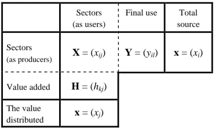
2.1. Applied input-output models ... - 42 -

2.1.1. The input-output table and Leontief’s static model ... - 42 -

2.1.2. Representation of foreign trade in the I-O tables ... - 44 -

2.1.3. Partial closure and extensions of the input-output models ... - 49 -

2.1.4. Applied input-output volume models ... - 50 -

2.1.5. Applied input-output price models ... - 54 -

2.2. Multisectoral resource allocation models: optimum versus equilibrium ... - 62 -

2.2.1. Linear optimal resource allocation models for economic policy analysis ... - 62 -

2.2.2. Ad hoc bounds in linear models to constrain overspecialization ... - 65 -

2.2.3. Flexible versus rigid individual bounds: nonlinear approach ... - 68 -

2.2.4. Conclusions: towards the computable general equilibrium models ... - 76 -

2.3. The concept and the main building blocks of the CGE models ... - 81 -

2.3.1. From programming to applied equilibrium model... - 81 -

2.3.2. A stylised CGE model based on problem 2.2-2 ... - 83 -

2.3.3. Counting equations and variables and closing the CGE model ... - 88 -

2.3.4. Notes on the calibration of substitution functions used in the CGE model . - 92 - 2.4. Illustrative programs ... - 100 -

3. The specific features of the GEM-E3 model ... - 101 -

3.1. Household’s behaviour ... - 103 -

3.2. Firms’ behaviour ... - 107 -

3.3. Government’s Behaviour ... - 111 -

3.4. Domestic demand and trade flows ... - 112 -

3.5. Equilibrium pricing identities ... - 115 -

3.6. The income distribution and redistribution block ... - 115 -

3.7. Market clearing conditions ... - 119 -

3.8. Model Calibration and Use ... - 121 -

4. Extensions of the GEM-E3 core models ... - 123 -

4.1. The environmental module ... - 123 -

4.1.1. Mechanisms of emission reduction ... - 125 -

4.1.2. The firm's behaviour ... - 125 -

4.1.3. The consumer's behaviour ... - 126 -

4.1.4. End-of-pipe abatement costs ... - 126 -

4.1.5. User cost of energy ... - 128 -

4.1.6. Abatement decision ... - 129 -

4.1.7. The ‘State of the Environment’ module ... - 131 -

4.1.8. Instruments and policy design ... - 133 -

4.2. Multiple households ... - 135 -

4.3. Illustrative programs ... - 137 -

5. Statistical background of the GEM-E3 model ... - 138 -

5.1. The primary data requirements of the model ... - 138 -

5.2. Sources of the primary data ... - 141 -

5.3. Data availability and problems ... - 144 -

5.4. Data processing methods ... - 147 -

5.4.1. Processing the Input-Output table ... - 148 -

5.4.2. The compilation of the other blocks of the GEM-E3 SAM. ... - 150 -

5.4.3. The baseline emission coefficients ... - 155 -

5.5. Techniques for estimating the missing data ... - 156 -

5.5.1. Using proxies: ... - 156 -

5.5.2. Computing as residual: ... - 156 -

5.5.3. Routing through ... - 156 -

5.5.4. ‘Rooking’ ... - 156 -

5.5.5. Miniature programming methods ... - 156 -

5.6. Techniques for the reconciliation (adjustment techniques) of inconsistent data .. - 157 -

5.6.1. The RAS-method ... - 157 -

5.6.2. The ‘additive’ RAS-method ... - 158 -

5.7. Summary ... - 159 -

6. Compilation of the database for the GEM-E3 model: the example of Hungary ... - 160 -

6.1. Domestic output and imports ... - 160 -

6.2. Indirect taxes ... - 161 -

6.3. Investment transformation matrix ... - 162 -

6.4. Consumption transformation matrix ... - 162 -

6.5. Accounting for tourism ... - 163 -

6.6. The Social Accounting Matrix (SAM) ... - 164 -

6.7. Bilateral trade matrix ... - 167 -

6.8. Energy balance sheets ... - 171 -

6.9. Emission data ... - 171 -

7. Implementation of the GEM-E3 model ... - 173 -

7.1. The GAMS software ... - 173 -

7.2. Reading in the data from CSV files and Excel tables ... - 175 -

7.2.1. Import data from Excel to GAMS ... - 175 -

7.2.2. Export data from GAMS to Excel ... - 178 -

References ... - 183 -

APPENDIX 1: The I-O table in GEM-E3 nomenclature ... - 191 -

APPENDIX 2: Correspondence between NACE and external trade product code ... - 193 -

APPENDIX 3: The derivation of symmetric I-O tables... - 194 -

APPENDIX 4: The Consumption Matrix of Greece ... - 197 -

APPENDIX 5: The United Kingdom Investment Matrix ... - 197 -

APPENDIX 6: Models of Optimal Resource Allocation ... - 199 -

Introduction ... - 199 -

Formal description of the models ... - 199 -

The NLP2 (primal optimal resource allocation) model ... - 199 -

The NLP3 model (first order conditions of the NLP2 model) ... - 201 -

The NLPKT model (modified version of the first order conditions) ... - 204 -

The NLPGE model (slightly modified NLPKT) ... - 206 -

The CGE and CGECLO models (toward a general equilibrium model) ... - 206 -

APPENDIX 7: Flow chart of the Hungarian CGE model ... - 208 -

CGE Modelling: A training material

Introduction

Computable General Equilibrium (CGE) modelling is an attempt to use general equilibrium theory as an operational tool in empirically oriented analyses of resource allocation and income distribution issues. Economic theory helps to understand conceptually the linkages between trade, income generation, employment, and the effect of government policies.

The distinguishing features of general equilibrium modelling derive from the Walrasian general economic equilibrium theory that considers the economy as a set of agents, interacting in several markets for an equal number of commodities under a given set of initial endowments and income distribution. Each agent defines individually his supply or demand behaviour by optimizing his own utility, profit or cost objectives. His decision yields a set of excess supply functions that fulfil the Walras law, i.e., the global identity of incomes and expenditures. Arrow and Debreu (1954), McKenzie (1954) and others have proved that under some general conditions, there exists a set of prices that bring supply and demand into equilibrium.

Computable general equilibrium (CGE) models turned the above theory into an operational model to be used for comparative static analysis. CGE models determine simultaneously changes in quantities of goods supplied and demanded, and their prices, in an aggregated multi-sectoral and multi-agent setup. Facilitated by the explicit representation of markets, the CGE models have been often extended beyond the original Walrasian framework to model market imperfections and other economic mechanisms that deviate from the original general equilibrium paradigm. For this and similar other reasons, some authors used the term

“generalized equilibrium modelling” (Nesbitt, 1984) or “general equilibrium programming”

(Zalai, 1982a) to underline the flexibility of the computable general equilibrium models.

Salient CGE models

CGE models have grown out of and combine different modelling traditions. The first CGE model, L. Johansen’s Multisectoral Growth (MSG) model (Johansen, 1960) was built for Norway. The MSG model was a combination of the dynamic Leontief-type (input-output) model with macroeconomic production and consumption functions, thus extending the input- output model with relative price driven substitution possibilities. Many models followed or were inspired later by Johansen’s pioneering work both in Norway (see, for example, Longva, Lorentsen and Olsen, 1985) and elsewhere (see, for example, the ORANI model in Australia, Dixon et al., 1982).

In a related but somewhat different approach D. Jorgenson and his associates combined the input-output model with macro functions based on the econometric tradition (see, Hudson and Jorgenson, 1974 and 1977, Jorgenson, 1984, Jorgenson and Wilcoxen, 1990a and 1990b).

The work of Jorgenson has also inspired many modelling efforts, in which particular emphasis has been put to issues related to energy and environmental policy (see, for example, Bergman, 1988 and 1990, Capros and Ladoux, 1985, the OECD, 1994 GREEN model, Conrad and Henseler-Unger, 1986).

The 1970s and the 1980s witnessed a widespread use of CGE models for the analysis of economic development problems of the developing countries (see, e.g., Adelman and Robinson, 1978, Dervis, De Melo and Robinson, 1982, Devarajan, Lewis and Robinson, 1987). These models have enriched the CGE modelling tradition extending the focus of the previous models with elaborate treatment of foreign trade, income distribution and various policy instruments. Many of these models have further departed from the Walrasian concept by including “structuralist” features into the general equilibrium framework (see, for example Taylor and Black, 1974, Taylor and Lysy, 1979). Modellers associated with the World Bank have animated a large number of modelling projects. Their work contributed to the standardization of the CGE approach: data base cantered around the Social Accounting Matrix (see, Decaluwe and Martens, 1988) and computer software packages for handling CGE models such as like GAMS, HERCULES, MPS/CGE.

A significant source of inspiration for CGE modelling was the competitive general equilibrium interpretation of the primal-dual solutions to linear programming (LP) models of nation-wide resource allocation. LP models were extensively used in the 1960s and 1970s for economic policy analysis, both in the developing and the centrally planned economies. A distinct method that developed from that tradition was the activity analysis approach to CGE models (Ginsburgh and Waelbroeck, 1981). The development of the HUMUS model family has also taken this point of departure, interpreting CGE models as natural “general equilibrium” extensions of the LP programming-planning models (see, Zalai, 1984a).

Harberger’s (1962) early numerical two-sector model analyzing the incidence of taxation and the pioneering work of Scarf (1973) presenting the first constructive method for computing fixed points initiated another distinct trend of general equilibrium modelling. It oriented chiefly towards the study of tax policy and international trade (see, for example, Shoven and Whalley, 1972 and 1984, Scarf and Shoven, 1984, Fullerton, King, Shoven and Whalley, 1981, Pereira and Shoven, 1988). Shoven and Whalley provided a state-of-the-art methodology for model calibration and formulating multi-national market clearing mechanisms in a general equilibrium framework.

A more recent trend in computable general equilibrium modelling consists in incorporating an IS-LM mechanism (termed also macro-micro integration) which has been traditionally used in Keynesian models. Bourguignon, Branson and De Melo (1989) and others have proposed the ensuing hybrid models. These models often incorporate additional features that enhance their short or medium term analysis features, such as, for example, financial and monetary constraints and rigidities in wage setting.

Another recent development was the incorporation of economies of scale and non- competitive (oligopolistic) market structures into the CGE framework, in order to model the effects of trade liberalization and integration on micro efficiency. The forerunner of these

models is a Harris’s (1984) pioneering work and the partial equilibrium model of Smith and Venables (1988). In the 1990s several models carried further this line of research, including Harrison, Rutherford and Tarr (1994), Willenbockel (1994), Burniaux and Wealbroeck (1992), Capros at al. (1997).

Thus, in the last 20 years or so, an enormous number of practically useful CGE models have been developed to study a wide range of policy areas in which simpler, partial equilibrium tools would not be satisfactory. Equilibrium models have been used to study a variety of policy issues, including tax policies, development plans, agricultural programs, international trade, energy and environmental policies and so on. A range of mathematical formulations and model solution techniques has been used in these modelling experiences.

The practice of model building itself became increasingly systematized, as reflected for instance, in the increasing use of standard and rather powerful packages such as GAMS.

The advantages of computable general equilibrium models for policy analysis compared to traditional macro-economic models are now widely admitted. The general equilibrium models allow for consistent comparative analysis of policy scenarios by standardizing their outcome around the concept of an equilibrium point, fulfilling the same consistency criteria.

In addition, the computable general equilibrium models incorporate micro-economic mechanisms and institutional features within a consistent macro-economic framework, and avoid the representation of behaviour in reduced form. This allows analysis of structural change under a variety of assumptions.

Several surveys are available in various handbooks and journals from different points of time and focusing on models developed for one or other specific purpose. We call attention to a few of them. “A Bibliography of CGE Models Applied to Environmental Issues” by Adkins and Garbaccio (1992) contains most of the relevant literature up to the beginning of 1990s. In their conceptual, theoretical review, “CGE Modeling of Environmental Policy and Resource Management” Bergman and Henrekson (2003) provide a more up-to-date account on the area that is of special concern of our study: analysis of the interrelation of energy, environment and economy. Table 1 lists the models and their main characteristics they have covered in their review. It provides a useful quick orientation of the most known modelling experiments and their characteristics for the interested reader. Ghersi and Toman (2003) have also put together a very informative summary of 15 models in their paper, "Modeling Challenges in Analyzing Greenhouse Gas Trading" (see Table 2). Finally, Francois and Reinert eds. (1997/98) annually update their table contained in "Applied Methods for Trade Policy Analysis: A Handbook", the last update (2004) of their summary table available on the WEB is reproduced as Table 3.

TABLE 1: KEY CHARACTERISTICS OF SELECTED GLOBAL AND REGIONAL E3 CGE MODELS (BERGMAN AND HENREKSON,2003)

Model Reference Regions Sectors per

region

Dynamics Energy sector Backstop technology

Technological change

Environmental benefits

WW Whalley and Wigle (1991) 6 3 Static Top-down No None Yes

GREEN Burniaux et.al. (1992) 12 11 Quasi-

dynamic

Top-down Yes AEEI No

Global 2100 Manne and Richels (1992) 5 2 Fully

dynamic

Bottom-up Yes AEEI No

12RT Manne (1993) 12 2 Fully

dynamic

Bottom-up Yes AEEI No

CRTM Rutherford (1992) 5 3 Quasi-

dynamic

Bottom-up Yes AEEI No

G-Cubed McKibbin et.al. (1995) 8 12 Fully

dynamic

Top-down No None No

MIT-EPPA Yang et.al. (1996) 12 8 Quasi-

dynamic

Top-down Yes AEEI No

RICE Nordhaus and Yang (1996) 13 1 Fully

dynamic

Energy a single prod. sector

Yes AEEI Yes

IIAM Harrison and Rutherford (1997) 5 2 Fully

dynamic

Top down No None No

ÚR Babiker et.al. (1997) 26 13 Static Top down No None No

MS-MRT Bernstein et.al. (1999) 10 6 Fully dynamic

Top down Yes AEEI No

AIM Kainuma et.al. (1999) 21 11 Quasi-

dynamic

Top-down No AEEI No

WorldScan Bollen et.al. (1999) 13 11 Quasi-

dynamic

Top-down No None No

GEM-E3 Capros et.al (1995)

(14 EU Member States and ROW)

15 18 Quasi-

dynamic

Top-down No AEEI Yes

BFR Böhringer et.al. (1998)

(Germany, France, UK, Italy, Spain, Denmark and ROW)

7 23 Static Top-down No - No

HRW Harrison et.al. (1989)

(US, Japan, France, Italy, UK, Ireland Germany, Netherlands, Belgium, Denmark, and ROW)

11 6 Static Top-down No - Yes

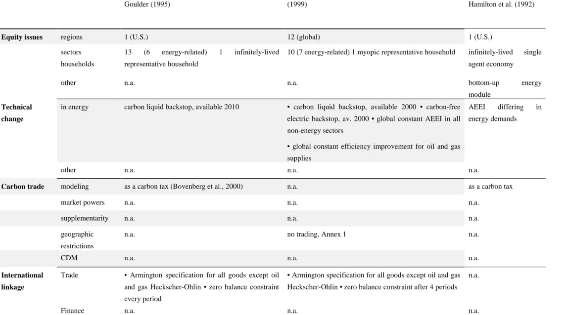
Table 2: Summary of Various Models (Ghersi and Toman, Appendix)

Goulder Goulder (1995)

EPPA (version 1.6) Yang et al. (1996) Jacoby et al.

(1999)

MARKAL-MACRO Hamilton et al. (1992)

Equity issues regions 1 (U.S.) 12 (global) 1 (U.S.)

sectors households

13 (6 energy-related) 1 infinitely-lived representative household

10 (7 energy-related) 1 myopic representative household infinitely-lived single agent economy

other n.a. n.a. bottom-up energy

module Technical

change

in energy carbon liquid backstop, available 2010 • carbon liquid backstop, available 2000 • carbon-free electric backstop, av. 2000 • global constant AEEI in all non-energy sectors

AEEI differing in energy demands

• global constant efficiency improvement for oil and gas supplies

other n.a. n.a. n.a.

Carbon trade modeling as a carbon tax (Bovenberg et al., 2000) n.a. as a carbon tax

market powers n.a. n.a. n.a.

supplementarity n.a. n.a. n.a.

geographic restrictions

n.a. no trading, Annex 1 n.a.

CDM n.a. n.a. n.a.

International linkage

Trade • Armington specification for all goods except oil and gas Heckscher-Ohlin • zero balance constraint every period

• Armington specification for all goods except oil and gas Heckscher-Ohlin • zero balance constraint after 4 periods

n.a.

Finance n.a. n.a. n.a.

MERGE

Manne et al. (1995, 1999), http://www.stanford.edu/group/MERGE/

SGM

MacCracken et al. (1999) Edmonds (1995)

G-CUBED

McKibbin et al. (1995, 1999)

Equity issues regions 5 (global), 9 (global) in MERGE 3.0 12 (global) 8 (global)

sectors households

infinitely-lived single agent economy 13 (11 energy-related) 1 myopic (?) representative household

12 (5 energy-related) 1 hybrid representative household

other 9 electric, 9 non-electric energy supplies in energy module n.a. n.a.

Technical change

in energy • 2 carbon-free electric backstops, av. 2010 (low cost) and 2020 (high cost) • carbon liquid backstop (high price) • global constant AEEI in the aggregated sector

sector-specific exogenous growth in total productivity rate for energy sectors

• global constant AEEI • region- specific exogenous growth in total productivity rate for energy sectors

other n.a. sector-specific exogenous growth in

total productivity rate

region-specific exogenous growth in total productivity rate

Carbon trade modeling regional endowments are traded on an interregional market as a carbon tax harmonized within trading limits

regional endowments are auctioned then traded on an interregional market

market powers supplementarity

buyer's and seller's market cap on trade (33% of targeted reductions for net buyers)

seller's market cap on trade (10% of targeted reductions for net buyers, exact compensation in actual domestic efforts for net sellers)

n.a. n.a.

geographic restrictions

no trading, Annex 1, global trading no trading, double bubble, Annex 1, global trading

no trading, double bubble, Annex 1, global trading

CDM supplies an exogenous 15% of observed global trading transactions global trading is provided as a limit of its benefits

n.a.

International linkage

Trade • oil, gas, coal, and the single output, plus energy-intensive goods (EIG) in MERGE 3.0 are perfectly substitutable • carbon permits are perfectly substitutable • zero balance constraint every period • international transport priced • S/D ratio of domestic EIG provide assessment of trade impacts n.a.

• all goods perfectly substitutable except distributed gas nontradable • possibility of fixed quantities or prices • zero balance constraint after a few periods n.a.

Armington specification for all goods, with sensitivity analysis on the elasticities global investment market, perfect in OECD, constrained elsewhere

Finance n.a. n.a. n.a.

RICE-99

Nordhaus et al. (1999a, b)

FUND (version 1.6) Tol (1999)

GRAPE

Kurosawa et al. (1999)

Equity issues regions 13 (global) 9 (global) 10 (global)

sectors households infinitely-lived single agent economy non-overlapping generations single agent economy infinitely-lived single agent economy

other n.a. n.a. bottom-up energy module

Technical change

in energy • carbon-free energy backstop (high price) • region-specific A Carbon EI in the aggregated sectors

• global AEEI in the aggregated sector • global A Carbon EI in the aggregated sector

• AEEI in the aggregated sector • oil substitutes in transports av. 2010 • nuclear substitute available 2050

other region-specific exogenous growth in total factor productivity in the aggregated sector

n.a. n.a.

Carbon trade modeling as a carbon tax harmonized within trading limits

as cooperation in a game-theoretic sense: sum of the welfares of the trading regions is maximized with actual regional reductions as control variables

as a carbon tax harmonized within trading limits, with a constant unit transaction cost of 1990$10 a ton

market powers supplementarity

n.a.n.a. n.a.cap on trade (10% of targeted reductions for net buyers, for net sellers, and for both jointly)

n.a. n.a.

geographic restrictions

no trading, OECD, Annex 1, global trading

no trading, double bubble, Annex 1, Annex 1 and Asia, global trading

no trading, Annex 1, global trading

CDM n.a. n.a. global trading has emissions outside

Annex 1 constrained to their no-trading level; CDM is not explicitly mentioned International

linkage

trade n.a. except single output in compensation of permits

n.a. • in single output • in energy products in

the bottom-up energy module

finance n.a. n.a. n.a.

WORLDSCAN

Bollen et al. (1999),

http://www.cpb.nl/nl/pub/pubs/bijzonder_20/

AIM

Kainuma et al. (1999)

http://www-cger.nies.go.jp/ipcc/aim/

MS-MRT

Bernstein et al. (1999)

Equity issues regions 13 (global) 21 (global) 10 (global)

sectors 11 (4 energy-related) 11 (7 energy-related) 6 (4 energy-related)

households overlapping generations 1 myopic representative household 1 infinitely-lived representative

household other? • high and low-skilled labour • region-specific unformal

(low-productivity) sectors

n.a. n.a.

Technical change

in energy other n.a. region- and sector-specific exogenous growth in factors productivity rate

• global constant AEEI • global constant A Carbon EI n.a.

• carbon-free backstop (high price) • AEEI growth in total factor productivity, endogenous returns on capital

Carbon trade modeling as a carbon tax harmonized within trading limits regional endowments are traded on an interregional market

regional endowments are traded on an interregional market

market powers

supplementarity

n.a.cap on trade (10, 15 and 25% of targeted reductions for net buyers, and for net sellers)

n.a.n.a. seller's market • cap on trade • ban on

"hot air"

geographic restrictions no trading, double bubble, Annex 1, global trading no trading, double bubble, Annex 1, global trading

no trading, Annex 1, global trading

CDM • financing of retrofit projects following a cost-benefit analysis with additionality constraint (cf. text) • exogenous 5% of targeted reductions

as global trading with emissions outside Annex 1 constrained to their BAU level

supplies an exogenous 15% of observed global trading transactions

International linkage

trade Armington specification for all goods turning to Heckscher- Ohlin in the long-run

• all foreign goods perfectly substitutable • Armington specification for domestic and aggregated foreign goods

• Armington specification for all goods except oil, electricity nontradable • trade balanced over time horizon • study of terms-of-trade variations

finance Imperfect global investment market perfect global investment market • zeroed on the growth path • perfect mobility of capital

GTEM

Tulpulé et al. (1999)

http://www.abare.gov.au/pdf/gtem.doc

OXFORD

Cooper et al. (1999)

CETA

Peck and Teisberg (1992, 1999)

Equity issues

regions 18 (global) 22 (mostly OECD), key macro variables for

50 more

2 (global)

sectors households

16 (5 energy-related) 1 myopic representative

households infinitely-lived single agent economy Infinitely-lived single agent economy other saving decisions (forward-looking) are

disaggregated in age groups

6 energy supplies, 4 energy demands in energy module for 8 regions

7 electric, 5 nonelectric energy supplies in energy module

Technical

change in energy endogenous n.a.

• nonelectric and electric carbon-free backstops (high prices) • global constant AEEI in aggregated sector

other endogenous

region-specific growth in total factor productivity, exogenous trend corrected by energy prices ("crowding-out wise")

n.a.

Carbon trade

modeling as a carbon tax harmonized within trading limits, with impact on GNP

as a carbon tax harmonized within trading limits, with impact on GNP

Regional endowments are traded on an interregional market

market powers n.a. n.a. n.a.

supplementarity n.a. n.a. n.a.

geographic

restrictions no trading, double bubble, Annex 1 no trading, double bubble without trade in

the EU, Annex 1 Annex 1, global trading

CDM n.a. n.a. n.a.

International

linkage trade

• Armington specification for all goods • international transport priced

Armington specification for the single output Carbon permits, the nonenergy good, oil and gas, and synthetic fuel are perfectly substitutable

finance imperfect global investment market perfect global investment market n.a.

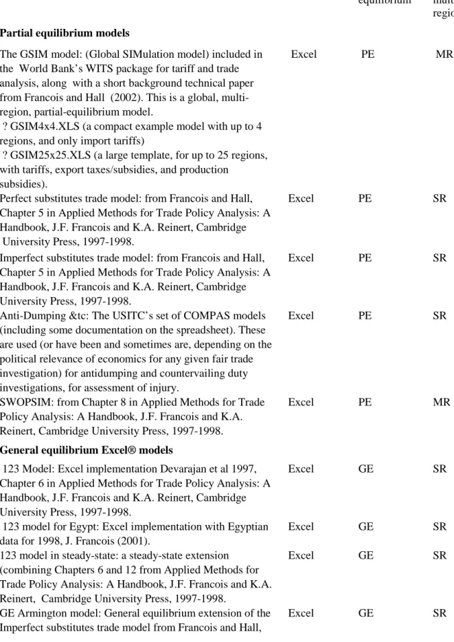
Table 3: Calibration-based numerical trade policy models (Francois and Reiner, 2004)

Description Software

required

Partial or general equilibrium

Single or multi- region Partial equilibrium models

The GSIM model: (Global SIMulation model) included in the World Bank’s WITS package for tariff and trade analysis, along with a short background technical paper from Francois and Hall (2002). This is a global, multi- region, partial-equilibrium model.

? GSIM4x4.XLS (a compact example model with up to 4 regions, and only import tariffs)

? GSIM25x25.XLS (a large template, for up to 25 regions, with tariffs, export taxes/subsidies, and production

subsidies).

Excel PE MR

Perfect substitutes trade model: from Francois and Hall, Chapter 5 in Applied Methods for Trade Policy Analysis: A Handbook, J.F. Francois and K.A. Reinert, Cambridge University Press, 1997-1998.

Excel PE SR

Imperfect substitutes trade model: from Francois and Hall, Chapter 5 in Applied Methods for Trade Policy Analysis: A Handbook, J.F. Francois and K.A. Reinert, Cambridge University Press, 1997-1998.

Excel PE SR

Anti-Dumping &tc: The USITC’s set of COMPAS models (including some documentation on the spreadsheet). These are used (or have been and sometimes are, depending on the political relevance of economics for any given fair trade investigation) for antidumping and countervailing duty investigations, for assessment of injury.

Excel PE SR

SWOPSIM: from Chapter 8 in Applied Methods for Trade Policy Analysis: A Handbook, J.F. Francois and K.A.

Reinert, Cambridge University Press, 1997-1998.

Excel PE MR

General equilibrium Excel® models

123 Model: Excel implementation Devarajan et al 1997, Chapter 6 in Applied Methods for Trade Policy Analysis: A Handbook, J.F. Francois and K.A. Reinert, Cambridge University Press, 1997-1998.

Excel GE SR

123 model for Egypt: Excel implementation with Egyptian data for 1998, J. Francois (2001).

Excel GE SR

123 model in steady-state: a steady-state extension (combining Chapters 6 and 12 from Applied Methods for Trade Policy Analysis: A Handbook, J.F. Francois and K.A.

Reinert, Cambridge University Press, 1997-1998.

Excel GE SR

GE Armington model: General equilibrium extension of the Imperfect substitutes trade model from Francois and Hall,

Excel GE SR

with a short background technical paper from Francois and Hall (1998).

Shipping model: International trade with imperfect

competition in shipping, from Francois and Wooton (2001),

“Market Structure, Trade Liberalization, and the GATS,”

European Journal of Political Economy.

Excel GE MR

GTAP: Dominique van der Mennsbrugghe’s spreadsheet implementation of the GTAP model.

Excel GE MR

General equilibrium models in GAMS® and GAUSS®

GTAP-E: A GAMS implementation of a model of

international trade that includes carbon emissions. You will need access to the GTAP database (not provided here). This version is for GTAP4, which is benchmarked to 1995.

GAMS GE MR

IFPRI standard model: This is the standard model developed by Sherman Robinson et al. when at IFRPI.

GAMS GE SR

123 Model: GAMS implementation of the 123 model from Devarajan et al 1997, Chapter 6 in Applied Methods for Trade Policy Analysis: A Handbook, J.F. Francois and K.A.

Reinert, Cambridge University Press, 1997-1998

GAMS GE SR

Single region U.S. CGE model: (from Chapter 7 of J.F.

Francois and K.A. Reinert, Cambridge University Press, 1997-1998.)

GAMS GE SR

Transition dynamics: a model of the Austrian economy from Chapter 13 in Applied Methods for Trade Policy Analysis: A Handbook, J.F. Francois and K.A. Reinert, Cambridge University Press, 1997-1998.

GAUSS GE SR

Labor markets in GE: from Chapter 14 in Applied Methods for Trade Policy Analysis: A Handbook, J.F. Francois and K.A. Reinert, Cambridge University Press, 1997-1998.

GAMS GE SR

The Small model: a 3-region model implemented in MPSGE. This is the same aggregation used for the

“SIMPLE” model below. HTML-based documentation is available.

GAMS GE SR

The Large Model: a multi-region, MPSGE-based model used while I was at the GATT/WTO to assess the Uruguay Round agreements. This model is SAM-based (our global SAM is included). This was published, in various forms, e.g,:

Francois, J.F. B.J. McDonald, and H. Nordstrom (1996),

"The Uruguay Round: A Numerically Based Qualitative Assessment," in W. Martin and A Winters, eds., The Uruguay Round and Developing Countries, Cambridge Univesity Press.

This includes a number of features that were innovative for CGE models once upon a time: (1) explicit quotas (included in the file), (2) global monopolistic competition, and (3) steady-state investment effects (included in the file, and called “numeric ballistics” by Glenn Harrison when he first commented back in 1993).

GAMS GE MR

General equilibrium models in GEMPACK®

GTAP model (old version): from Chapter 9 in Applied Methods for Trade Policy Analysis: A Handbook, J.F.

Francois and K.A. Reinert, Cambridge University Press, 1997-1998.

This is a multi-region CGE model. Further documentation is available from

Chapter 2 of Hertel, T. (1996), Global Trade Analysis, Cambridge University Press.

GEMPACK GE MR

Steady-state investment effects: from Chapter 12 in Applied Methods for Trade Policy Analysis: A Handbook, J.F.

Francois and K.A. Reinert, Cambridge University Press, 1997-1998.

GEMPACK GE MR

Imperfect competition in GTAP: from J. Francois, Scale Economies and Imperfect Competition in the GTAP Model, GTAP Technical Paper No. 14, 1998.

GEMPACK GE MR

Capital accumulation in GTAP: from J. Francois, B.

McDonald, and H. Nordstrom, , Liberalization and Capital Accumulation in the GTAP Model, GTAP Technical Paper No. 07, 1996.

GEMPACK GE MR

The SIMPLE model:

This is a self-contained (i.e. executable) somewhat-dated version of the GTAP model. It includes scale economies, imperfect competition, nested- and non-nested import demand, rigid wages, and some capital mobility treatment.

The idea is to follow a single experiment across different model features. HTML-based documentation is available.

These examples are built on the same dataset as the “Small”

model in GAMS/MPSGE linked above.

GEMPACK GE MR

Purpose and organization of the monograph

This monograph is part of the effort to increase the capacity to apply multisectoral models for economic policy analysis, especially lacking in the New EU Member States, where such models have been missing from both university curricula and practice. As a result, there are hardly any experts in these countries knowledgeable or experienced in multisectoral modelling methodology widely used in a variety of areas of economic policy analysis in other parts of the world. The proper use of CGE models requires substantial knowledge and skills in several fields, including economic theory, statistics and computation techniques. The monograph was tailored first of all to the needs of students, research assistants and modellers coming from this environment, but might be useful additional reading for other interested beginners in the field elsewhere too. The monograph is supplemented by various computer programmes to provide numerical illustration and models to the themes presented.

This training material has been organized into chapters and sections as follows. The first chapter reviews and deepens the reader’s knowledge of the theoretical and methodical foundations of general equilibrium models necessary for the proper understanding of the

strengths and weaknesses of general equilibrium analysis. It is especially designed for those who have not studied in a systematic fashion mathematical economics and the history of economic thoughts.

It starts with two abstract models developed by Walras to explain concepts such as Walras law, price homogeneity, counting equations and macro-closure that reappear in the CGE models. The use of simpler models facilitates the understanding of those concepts and provides a useful introduction to the art of CGE model building. We also touch upon the issue of the use of weak inequalities and complementary restrictions in the market clearing conditions as well as the structural and reduced forms of the models by invoking the Cassel and Schlesinger-Wald variants of the first model of Walras.

The models presented above were stylized theoretical models not intended for practical application. Unlike those models Leontief developed the first applied general equilibrium model for policy analysis, the model of interindustrial or input-output analysis. In the third section the basic concepts and equilibrium conditions of Leontief’s model are introduced and discussed.

The early models of general equilibrium were holistic, macroeconomic models, not using any behavioural explanation for the determination of the choice of technology or final use. The pioneering works of Hicks and Samuelson filled this gap by merging the holistic, macro- economic framework with the neoclassical theories of firms and consumers. That approach became the framework of modern applied general equilibrium models. Section 1.4 describes the main components and conditions of general equilibrium in a model based on micro- economic foundations (differentiable production and utility functions).

The functions used in the neoclassical GE model however are not easy to estimate in the practice. Modellers therefore had to circumvent often the problem by using an alternative representation of technology and preferences based on the use of fixed coefficients and linear relationships. Koopmans and Kantorovich were awarded for laying down the theoretical and methodological foundations of applied linear economic models. In section 1.5 we discuss the basic concepts and theorems of linear activity analyses, which form the basis of the linear programming (LP) approach used extensively in the analysis of resource allocation. The nation-wide LP models can be interpreted as linear GE model. We illustrate that point by presenting a Koopmans–Kantorovich type model of general equilibrium that is the linear equivalent of the Hicks–Samuelson GE model presented in the previous section.

In section 1.6 we pave further the way leading to modern CGE models by presenting a stylized version of the first applied general equilibrium model developed by Leif Johansen.

This model is a combination of Leontief-type input-output model with macroeconomic production and consumption functions, thus an input-output model extended with relative price driven substitution possibilities. Many models followed or were inspired later by Johansen's pioneering work and retained its original structure. In order to keep the model transparent, we present a prototype version of the model with no foreign trade and taxes, and with no income redistribution.

Finally, the last section summarizes the models presented and discussed in order to ease their survey and comparison.

The chapter is accompanied by two numerical examples and exercise package. The first is an Excel realization of the Cassel-model assuming 2 factors and 3 products (Cassel-2x3.xls and Cassel-2x3.doc). This exercise illustrates how the neoclassical theory works in practice and how the equilibrium solution depends on the parameters of the model. The second is an Excel illustration of the simplified Johansen CGE model (Johansen-DinLeo.xls). This program demonstrates also how simpler CGE models can be solved by iterating only with a few variables and repeatedly solving a set of simultaneous equations.

In the second chapter the main variants of applied multisectoral models macroeconomic models, the input-output, linear programming and computable general equilibrium approach discussed and compared with each other. Special emphasis is laid on their close similarity and features which link them together. The systematic review and discussion of the alternative macroeconomic multisectoral models reveals their common features and differences. The comparative analysis of the various model types is a crucial step in the explanation of the CGE approach especially for modellers coming from the former socialist countries. It enables the reader (student) to understand better the general philosophy lying behind the computable general equilibrium approach and models. In the training seminar we could see that it was considered to be very useful even for students who have acquired already some experience in building and running CGE models.

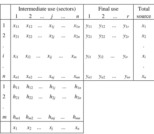
In the first section the basic concept and content of the statistical input-output tables (one of the main data source of the CGE models), and their relation to Leontief’s static input-output model are reviewed. Next we discuss the alternative ways in which foreign trade can be represented in the I-O tables. The partial closure possibilities and possible extensions of the input-output models prepare the ground for the presentation of complex volume and price models, which reappear as product balance and equilibrium pricing conditions in the computable general equilibrium models as well, not only un the pure input-output models.

The second section deals with the optimal resource allocation models taking the form of a linear or nonlinear programming problem and based on an input-output technology. By means of simple models we discuss in brief how optimal resource allocation models can be used for economic policy analysis. We point out to the basic problem of the linear programming approach, namely that these models tend to produce unrealistic overspecialized solutions. The only way to constrain overspecialization in a linear model is the introduction of ad hoc bounds on certain groups of variables, which in turn distorts the shadow prices of the commodities and resources on the other hand.

We demonstrate next that the use of rigid bounds is equivalent to assume less then perfect substitution between certain pairs of commodities in use or production represented by piece- wise linear isoquants or indifference curves. Switching to smooth, differentiable curves one can arrive at a nonlinear version of the same resource allocation problem that uses ‘flexible’

rather than rigid bounds to constrain specialization. The nonlinear model produces much more meaningful prices for the commodities and resources appearing in the model.

It is pointed out that the first order necessary conditions of the optimal solutions of a nonlinear resource allocation model – using appropriate functional forms – resemble the conditions of general equilibrium. There can be only a few conditions which will have to be revised and changed in order to get the conditions of a perfect competitive equilibrium.

Introducing taxes and subsidies in appropriate places into the set of equilibrium conditions one can arrive at a stylized CGE model.

In the third section the main building blocks of the CGE models are introduced and discussed: the commodity structure, representation of technology and production decisions, the representation of exports and imports, income distribution and final demand (consumption and investment), and market clearing equilibrium conditions. We close the section and the chapter by discussing the CES functional forms typically used in CGE models, and their calibration procedure.

This chapter is also accompanied by exercise programmes and materials. To facilitate the understanding of the characteristics of the programming models we developed an Excel program (LP-2x2-6eset-CES.xls), which computes and graphically displays the feasible set, the main functions and the optimal solution. The use of a CES welfare function helps also the user to understand the nature and role of CES functions in CGE-models. The program also illustrates the sensitivity analysis of the multisectoral macroeconomic models.

Another exercise possibility is provided by a GAMS model that distinguishes 3 sectors and 10 household groups, and was calibrated using Hungarian data for 1998 (MultHH-opt- scen.GMS). The model, by setting appropriately the value of certain parameters, can be used for the solution of both an NLP and CGE variant of the same problem and for the comparison of their behaviour. We have also developed an Excel interface for this GAMS program, which can present and compare the results of up to 7 simulation runs in a transparent Excel format.

The GAMS code of this program provides thus a useful exercise that teaches the user how to present model results in Excel.

Having prepared the ground in this way, in chapter 3 we turn to the detailed presentation of the specific features of a typical GEM-E3 model in the third chapter. We go through one by one the issues related to the assumed household’s, firm’s and government’s behaviour, domestic demand and trade flows, the equilibrium pricing identities, the representation of income distribution and redistribution, the market clearing conditions. We pay special attention to the issues related to model calibration and use in economic policy analysis.

Extensions of the GEM-E3 model include the generalization of the household utility function to take into account of the geographic variety of consumer goods, imperfect competition, the financial module determining the general price level, etc. In the training material we presented only the environmental module and discussed the possibility of representing private consumption and income generation with multiple households.

Chapter 4 describes two important extensions of the GEM-E3 model. In the first section the environment module is introduced, which represents the effects of different environmental policies on the economy and the state of the environment. It concentrates on three important

environmental problems: (i) global warming (ii) problems related to the deposition of acidifying emissions, and (iii) ambient air quality.

Next, the three components of the environmental module are described in details. Namely, the “behavioural” module representing the effects of different policy instruments on the behaviour of the economic agents, a “state of the environment” module, and the “policy- support component”, including the policy instruments related to environmental policy.

The three mechanisms that affect the level of actual emissions in the model: (i) end-of-pipe abatement technologies (ii) Substitution of fuels, and (iii) production or demand restructuring between sectors and countries are also explained in some details.

The presentation of the GEM-E3 model’s environmental module was accompanied by a model developed for Hungary, which was based on the extension of the GEM-E3 environmental module.

The second section describes the problems that arise, when multiple households and their relationships with the labour market and income distribution are represented in a CGE model.

After discussing the various socio-economic group-formation criteria, we present a neoclassical quasi-dynamic CGE-model. The model was calibrated for Hungary and distinguishes 3 sectors and 10 household groups (MULTHH.GMS program). The model contains group specific human capital (accumulated by the “productive” use of the household expenditure) and group specific financial wealth. CET-labour supply functions and alternative closures rules increase the flexibility of the model in policy analysis. This program allows also for useful practical exercises.

The fifth chapter is devoted to the issues related to the statistical background of the GEM- E3 models. In order to calibrate the parameters of a GEM-E3 model one has to compile benchmark year data on the production technology (incl. emission of air pollutants), consumption patterns, taxes, income distribution, savings and final demands. These data can be derived from various sources. The following data, their availability and method of estimation or derivation is discussed in details in this chapter:

− I-O tables and their supplementary tables, the import matrix and the matrix of indirect taxes and subsidies, import duty matrix;

− foreign trade matrices (exports and imports by commodity groups and partner countries);

− consumption transformation matrix;

− investment matrix;

− income distribution data, such as like the value added and its primary distribution /wages, social security, production taxes, production subsidies, operating surplus, income- expenditure balance sheets;

− environmental data needed for GEM-E3, for example, emission coefficients per type of activity for the pollutants considered in the model, marginal abatement cost functions for some of the pollutants, coefficients representing pollutants’ transformation and transportation between countries, damage per pollutant and its monetary valuation;

− auxiliary data, such as like factor endowment data, interest rates, inflation rate in the base year, demographic data, foreign tourists domestic consumption expenditure by supplier branches and the related VAT and consumption tax, energy balance sheets, energy taxes, stocks of energy consuming durable goods, share of gasoline and gas-oil within motor-fuel demand, share of non-energetic use of the energy carriers, etc.

The GEM-E3 model distinguishes 18 branches, 13 consumption categories, the list of which and their content can be seen in the tables of Appendix 1 of the training material. The method of reclassification (aggregation) from the original break-downs to the desired break- downs can be found in Appendix 2. Since most of the above data enter into a SAM (Social Accounting Matrix) scheme, designed specially for the GEM-E3 model, this chapter gives a detailed description of the SAM and instructions how to fill it with the available data.

A separate appendix contains an extract of the SNA 1968 volume’s method for the compilation of the Input-Output tables from the so called ‘Make’ and ‘Use’ tables. To illustrate this method in a simplified case, in this chapter we present an Excel-worksheet (MakeUse.XLS file) elaborated for the Hungarian CGE model. Several special programmes developed for these purposes of estimating missing data, reconciling and aggregating the available data (e.g., the flexible and general aggregation-reclassification program or the ‘additive-RAS’ algorithm) are also presented.

Chapter 6 describes step by step and in great details how the Hungarian data were compiled for the GEM-E3 model in order to illustrate the whole process. The compilation of the income distribution block of the SAM is discussed in the greatest detail, drawing useful conclusions for a similar process for other countries. This special emphasis is justified by the fact that the data availability and methodology of the income distribution is rather different across countries, so it is important to demonstrate how we can overcome these problems especially in new EU- countries where income distributional data are the least accurate and detailed.

Chapter 7 outlines the model implementation process. The latest versions of the GEM-E3 model involve systems of about 60,000 non-linear equations per time period. The GEM-E3 model has been successfully transformed into a mixed complementarity model and solved in GAMS using the PATH solver. Previous attempts to solve the model in other solution algorithms (as with MINOS and CONOPT) have been unsuccessful mainly due to the model’s large size and complexity. The PATH solver on the other hand, has been successful in solving very large scale models and through the complementarity approach that it uses, enables the expansion of GEM-E3 to include inequalities and a separate optimisation energy sub-module.

The www.gams.com website contains the documentation and the system files of the GAMS package. The GAMS is a rather efficient and model-builder friendly software to handle and solve large nonlinear models with ’well-behaving’ (twice differentiable, etc.) functions in its equations. Several sample programs are used to explain and illustrate the structure of the GAMS programmes and highlight the main syntactic rules which are important from the point of view of the GEM-E3 model’s program.

1. Salient models of general equilibrium

1.1. The static Walras–Cassel model of general equilibrium

Walras modelled the exchange of commodities at macro level, as if it would take place only between two agents, one representing the households and the other the firms (producers).

The exchange taking place between various households or producers is thus left out of consideration. Households own all stocks and resources, including the factors of production, and demand produced goods for consumption. At a given set of product and production factor prices they decide on the supply of factors and the demand for goods. Walras assumes that their choice can be represented by two sets of demand-and-supply functions: demand functions for the produced goods, v_i(p, r), i = 1, 2,…, n and supply functions of the factors of production, s_k(p, r), k = 1, 2,…, s. The nomenclature used is the following: n is the number of products (final goods), s is the number of primary resources, p = (pi) and r = (rk) are the price vectors of products and primary resources, respectively.

Walras assumes that the household’s demand and supply functions are homogeneous of degree zero (only price ratios matter) and always fulfil the budget constraint, that is, the total value of demand equals that of supply (the so called Walras’s law):

∑i pi⋅vi(p, r) = ∑k rk⋅sk(p, r).

Firms possess nothing, but merely organize production by demanding factors from households and supplying produced goods. Production technology is represented by fixed dkj

coefficients, which indicate how much factor k is used (on average) to produce one unit of final output j. At any given set of prices, firms produce only those commodities, the prices of which cover or exceed their cost of production. Walras assumes that no profit can be earned in perfectly competitive equilibrium, for any profit would lead to bidding up the prices of some factors of production. In equilibrium, therefore, prices have to meet the requirements of the so- called non-profit pricing rule:

p_j = r₁·d_1j + r₂·d_2j +…+ r_s·d_sj, j = 1, 2,…, n. (WS-1) where the variables are

p_i unit price of product i (i = 1, 2,…, n), rk unit price of factor k (k = 1, 2,…, s).

The further conditions of general equilibriumin the static Walras model are the supply- demand equations on the product markets:

v_i(p, r) = y_i, i = 1, 2,…, n, (WS-2)

where yi is the (final) output of product i (i = 1, 2,…, n), and on the factor markets:

dk1·y1 + dk2·y2 +…+ dkn·yn = sk(p, r), k = 1, 2,…, s. (WS-3) The three sets of equations contain 2×n + s variables (unknowns). However, because of the assumed homogeneity of the demand and supply functions and the price formation rule, the

price level is left undetermined by the above set of equations. It can be assigned any positive value, e.g., by selecting some commodity as numeraire good and setting its price to one. The total number of equations seems to exceed that of unknowns, and the model over-determined therefore.

We can however remove one equation by Walras's Law. Multiplying the equations with their complementing variables, yj, pi and rk, respectively and summing them up, after some rearrangement we get:

∑i pi⋅vi(p, r) = ∑k rk⋅sk(p, r),

which is the above introduced Walras’s Law? In other words: if all markets clear but one, then that last one will have to clear too. Thus, we can drop one of the market-clearing conditions out of the model. Thus, the number of equations becomes also 2×n + s – 1, equal to the number of the unknowns.

Although the equality of the number of equations and variables is neither necessary, nor sufficient condition for solution to exist, for Walras and his contemporaries this guaranteed that the model was consistent with the concept of equilibrium. This type of equation counting was not meant to prove the existence of equilibrium, as it is often falsely interpreted nowadays, but enough to prepare the ground for parametricising and calibrating the model in such a way that its solution would replicate the observed state of the economy concerned.

CASSEL’S VARIANT OF THE STATIC WALRAS MODEL

The Swedish economist, Cassel (1918) illustrated with almost the same set of equations the concept of general equilibrium as Walras, apparently independently from him. He ignored factor supply functions and assumed that all factors are supplied inelastically by agents, or better to say, by nature (primary resources). The final demand for produced goods in his formulation was function of their prices alone:

p_j = r₁·d_1j + r₂·d_2j +…+ r_s·d_sj, j = 1, 2,…, n. (C-1)

y_i(p) = y_i, i = 1, 2,…, n, (C-2)

d_k1·y₁ + d_k2·y₂ +…+ d_kn·y_n = s_k, k = 1, 2,…, s. (C-3) This set of conditions can be derived from a model consisting of equations (C-1), (C-2’), (C-3) and (C-4), where

y_i(p, e) = y_i, i = 1, 2,…, n, (C-2’)

e = ∑_k r_k⋅sk, (C-4)

where e is the expenditure (income) of the housholds and the y_i(p, e) demand functions are homogeneous of degree zero and satisfy a generalized form of Walras’s law: ∑_i p_i⋅y_i(p, e) = e.

Setting e = 1 as numaraire, and dropping (C-4) we arrive at Cassel’s form.

This model can easily be reduced further. Equations (C-1) define the p_j product prices as functions of the factor prices. Substituting the p_j variables with the resulting p_j(r) functions in equation (C-2) we can express all y_i as functions of r. Finally, substituting y_i variables in equation (C-3) by the resulting y_i(r) functions the demand for factors can be expressed as