(Kutatási beszámoló, MM-2016-4) Centre for Public Administration Studies Corvinus University of Budapest Hungary
F OREIGN TRADE IN MACROECONOMIC MODELS :
PROGRAMMING VERSUS GENERAL EQUILIBRIUM
Ernő Zalai and Tamás Révész
Content
1. Introduction ... - 1 -
2. Programming Models with Rigid Individual Bounds ... - 3 -
2.1. The Issue of Overspecialization ... - 3 -
2.2. Rigid Bounds on Export in a Simple Linear Programming Macroeconomic Model ... - 3 -
3. The Model with Flexible Bound Based on Export Demand ... - 5 -
4. The Model with Flexible Bound Based on Export Supply Function ... - 8 -
5. Equilibrium of Imperfectly Elastic Export Supply and Demand ... - 9 -
6. Export Supply Function Derived from Optimizing Decision ... - 13 -
7. Individual Bounds on Imports ... - 15 -
8. Equilibrium versus Optimum: Optimal Tariff Revisited ... - 18 -
9. Summing up: NLP versus CGE Model with Flexible Bounds ... - 19 -
10.Illustrative model simulations ... - 24 -
11.Conclusion ... - 30 -
REFERENCES ... - 31 -
Ernő Zalai – Tamás Révész
Foreign trade in macroeconomic models: Programming versus general equilibrium 1. INTRODUCTION
Multisectoral macroeconomic models fall roughly into three main classes: input-output (I-O) models, linear programming (LP) models, and general equilibrium (GE) models. In this paper we consider only models typical of the second and third classes, paying particular attention to the treatment of foreign trade, in these models.
The most important differences between the two modelling approaches examined here may be summarized as follows. The linear programming models contain mainly real (physical)
variables; most of their relations take the form of inequalities (balances and special restrictions) and contain as a rule quite a few individual bounds on certain variables.
Computable general equilibrium models, on the other hand, are specified in terms of both real and value (price and financial) variables, take the form of an equation system and include many nonlinear terms. The linear programming models optimize an overall objective (welfare) function, whereas in general equilibrium models distinguish various agents each optimization assume.
Despite these differences, computable general equilibrium models have many similarities to programming models. However, differences in the terminology used, conceptual and other difficulties have led to the impression that these two schools of macroeconomic modelling diverge rather than converge. LP models are tools designed for planning, whereas GE models for simulating the working of market economies. One of the authors (Zalai 1980, 1981) has demonstrated that – dispelling the neoclassical myth surrounding equilibrium models – computable general equilibrium models can be discussed in purely pragmatic terms, and they can be regarded as natural extensions of the programming models designed for planning.
This paper is concerned with the concepts of "equilibrium” and "optimum" in relation to export-import specification in macroeconomic models. In sections 2 and 3 we start by discussing the problem of overspecialization and possible methods of dealing with it in (linear) programming models as compared with computable general equilibrium models. The root of the problem is that most macroeconomic models adopt the common definition of small open economy, which implies that its terms of trade are dictated (fixed) by the world market.
It can be easily shown (see, for example, Taylor 1975) that exogenously fixed terms of trade tend to produce overspecialized solutions in linear macroeconomic models, basically due to the constant ratios of substitution implied by the linearity of the model. Overspecialization manifests itself in the existence of only a small number of producing and exporting sectors and allow for little or no intrasectoral trade. Such overspecialized solutions cannot be
defended on practical grounds. Thus, model builders must find ways to avoid such unrealistic solutions.
One can basically choose between two "pure” methods to prevent overspecialized solutions.
One, used in linear programming models, is to introduce special (upper and/or lower) bounds
on some important variables (e.g., sectoral output, export, import). The main criticism against this approach is that such bounds are rather arbitrarily chosen and influencing the solution.
The other method, offered by computable general equilibrium models, is to use nonlinear export-import relationships, which imply diminishing returns. The main aim of this paper is to show that the difference between these two approaches can be viewed as the choice using rigid (fixed) or flexible (variable) bounds on certain variables. Ginsburgh and Waelbroeck (1981), for example, argued on that ground that it would be natural and useful to include flexible bounds, by using piece-wise linear relations in linear programming models, instead of using fixed bounds.
The paper provides also a basis for discussing a number of other points. For example, to argue that it is necessary to make clear distinction between export restrictions caused by supply and demand limitations in computable general equilibrium models, which is not always the case.
A related issue is that export volume response to changes in relative prices is generally modelled by rather small export demand elasticities, which bring along unjustifiably large terms of trade effects. These problems call for a revision of common modelling practice in this field.
A related issue concerns the theoretical definition of small economies, which is incompatible with the assumption of less than perfectly elastic export demand. It is clearly inadequate to use this definition in applied models, since, due to market and product differentiation, even small countries face, as a rule, changing terms of trade as they change the volume of their exports. This has been realized by model builders and the use of less than perfectly elastic export demand as well as import demand functions is quite common. The theoretical justification is usually given as Armington's (1969) assumption of regional product differentiation.
Throughout of our discussion we will compare two modelling approaches used both in theoretical or applied macroeconomic policy analysis, the more traditional linear
programming and the general equilibrium models. This gives rise to the issue of optimum tariffs. From the theoretical literature on international trade it is known that the pure competitive (laissez-faire) equilibrium is not (Pareto) optimal for an economy which faces less than perfectly elastic export demand1 and optimum tariffs could be employed to produce optimal trade pattern in an otherwise competitive setting. This theoretical possibility is rightly neglected in the literature of computable (applied) general equilibrium models. The optimum tariffs, however, create a significant difference between the necessary conditions and the policy implications of the Pareto optimal and the laissez-faire equilibrium solution of the same resource allocation problem. The optimal solutions suggest rather severe import-export restrictions, whereas the laissez-faire solutions suggest a more open foreign trade policy. This problem will be briefly discussed in this paper too.
1 See, for example, Dixit and Norman (1980). See also Srinivasan (1982) for a theoretical discussion of this separation in a different context.
2. PROGRAMMING MODELS WITH RIGID INDIVIDUAL BOUNDS
2.1. The Issue of Overspecialization
It is well known that development planning models based on linear programming tend to suggest overspecialization, simply because the linear nature of the model implies either perfect substitutability or perfect complementarity between commodities or factors of
production. The most common means to prevent the model to extreme behaviour is to impose upper and/or lower bounds on different variables, particularly on production, export and import variables.
The use of individual bounds in linear programming planning models was not universally approved. One of the main criticisms is that they are ad hoc arbitrary restrictions, which can also distort the shadow-prices (see, for example, Taylor 1975, or Ginsburgh and Waelbroeck 1981). An alternative approach favoured by some model builders involves the introduction of more complicated nonlinear relationships into the model, perhaps in a piecewise linear fashion. We will come back to this possibility later.
The above criticism is, however, only partially justified. On the one hand, it is undoubtedly true that the individual constrains account for the inadequacy of the chosen model, reflecting our lack of knowledge and modelling ability. On the other hand, however, this problem, i.e., the arbitrariness of certain elements, is common to all economic models. In some models this is quite apparent, while in others it is partially hidden behind an elegant mathematical facade.
Thus, for example, the use of nonlinear relationships (rather than individual bounds) to limit overspecialization can just be seen as introducing another type of arbitrariness into the model.
Moreover, most of the individual bounds can be based on careful analysis of the underlying phenomena by experts; it is doubtful that this expertise could be replaced by some simple modelling device.
To avoid this argument becoming one-sided, we must make a brief mention of some points which will be discussed in more detail in later sections. It could be argued that the real choice is not between expert judgement and individual bounds, on the one hand, and nonlinear, econometrically estimated relationships, on the other. The parameters of the nonlinear forms in question could just as well be based on expert judgement as are the individual bounds in the other solution. Both solutions can provide equally realistic descriptions of the resource allocation problems analysed by the model.
In what follows it is argued that these nonlinear functions can be viewed as flexible bounds on certain variables. The main purpose of this and the next section is to demonstrate that most multisectoral computable general equilibrium models can be seen as programming models using flexible bounds. At the same time, through an illustrative example, some of the
deficiencies of shadow-prices and post-optimization analysis in the case of linear models are also pointed to.
2.2. Rigid Bounds on Export in a Simple Linear Programming Macroeconomic Model For the sake of simplicity an extremely stylized, textbook type of model will be used to open our discussion on the problem of overspecialization in linear models. Our attention is focused on the treatment of foreign trade. We assume that there is only one sector, whose net output
(Ȳ) is given (determined by available resources). Intermediate use will be neglected. The emerging allocation problem is how to divide Ȳ between domestic use (Cd) and export (Z), and how much to import, for the exported goods can be exchanged on the world market for import at given prices (pwe, pwm). The imported commodity is assumed to be perfect substitute for the home commodity. The goal is to maximize the total amount (Cd + Cm) by means of foreign exchange.
Following the traditional linear programming approach, export (pwe) and import (pwm) prices will be treated as (exogenously given) parameters in the model. Introducing M for the amount of imports purchased and Cm for the amount of imports used, our optimal resource allocation problem can be formulated in the following simple way:
LP I-II Primal problem Dual problem
Cd, Cm, Z, M 0 pd, pm, v, l, u 0
(pd) Cd + Z Ȳ pd 1 (Cd)
(pm) Cm M 0 pm 1 (Cm)
(v) pwm·M pwe·Z 0 pd v· pwe + l – u (Z)
(l, u) Žl Z Žu pm v· pwm (M)
Cd + Cm max! pd·Ȳ + u·Žu – l·Žl min!
where pd, pm, v and l, u are the dual variables associated with the constraints, i.e., the shadow-prices of domestic output, imports, foreign currency (shadow exchange rate), and of the individual lower and upper bounds on export, respectively.
In fact, two models are presented above, indicated by the broken line frames. Model I is defined by the variables and constraints other than those within frames, i.e., in which there are no individual bound prescribed for any variable. In the case of model II individual bounds (Žl
Z Žu, where Žu < Ȳ) constrain the volume of export. The solution of the above problems depends clearly on the relation of pwe and pwm, i.e., on the terms of trade.
In the case of Model I, if the terms of trade are favourable (pwe > pwm), total available home product will be exported (Z = Ȳ), and only imported goods will be consumed (Cd = 0, Cm = M
= pwe·Z/ pwm). All constraints will be binding, and the optimal values of the dual variables will be pm = 1, v = 1/ pwm, pd = pwe/ pwm. If the terms of trade are unfavourable (pwe < pwm), then the optimal policy will be autarky, i.e., Cd = Ȳ, Cm = M = Z = 0. pd = 1, 1/pwe v 1/pwm, 1 pm
v·pwm. In the case, when pwe = pwm, any solution exhausting available resources is optimal.
In the case of Model II the individual bounds set on export prevent such extreme solution as in Model I (everything or nothing). All primal variables (Cd, Cm, Z, M) will be positive, thus all dual constraints complementing them will become equalities in the optimal solution.
Depending on the terms of trade, the optimal volume of export will be either its upper bound (Z = Žu, if pwe > pwm) or lower bound (Z = Žl, if pwe < pwm). The case of pwe = pwm is a neutral case, any number between Žu and Žl is an optimal value for Z. Otherwise the solution is
Z = Žu or Žl, Cd = Ȳ – Z, Cm = M = pwe·Z/pwm;
pd = pm = 1, v = 1/pwm, l – u =1 – pwe/pwm, l·u =0 (one of them is zero).
As can be seen, in this simple model, the domestic prices of the domestically produced and imported commodity, which are assumed to be perfect substitutes, are equal, as they should be in perfect market equilibrium. The term l or u can be interpreted as a tax or subsidy on export, equalizing the income earned by the producer selling the home commodity on the domestic and foreign market. This is all in line with the working of a competitive market.
Introducing lower and upper bounds for Z forces thus its value stay within a “reasonable”
region, and thereby constrains the values of the other variables too. One could introduce individual bounds on the volume of the import too, or on its ratio to domestic supply, as will be discussed soon.
One of the problems of using simply lower and upper bounds (Žl, Žu) to limit the volume of export is that within these limits its changes are not influenced by any economic variable.
What is more, the export takes up, as a rule, one or the other extreme, arbitrarily fixed value.
This is basically caused by the linearity of the model used. In a nonlinear model it would be possible to make the volume of export depend on foreign and/or domestic variables.
3. THE MODEL WITH FLEXIBLE BOUND BASED ON EXPORT DEMAND
The analysis of such a model should not therefore stop here. The bounds set on export are estimated on certain estimated export price. If we changed pwe, these bounds would change too. A decrease in the export price, for example, would increase the export absorption capacity. So, instead of rigid lower and upper bounds, one could introduce, by means of an export demand function, Zd(pwe), a flexible upper bound, where the export price can change within certain limits itself. This would, however, turn our linear programming problem into a nonlinear one.
To keep the linear programming framework Srinivasan (1975) suggested to use piecewise linear functions. Another possibility would be to solve a series of linear programming, changing simultaneously the two parameters, Ž and pwe. If the export constraint is binding, it indicates that relaxing the constraint, even decreasing simultaneously pwe, would increase the value of the objective function. Thus, one could change, step by step, the value of parameters Ž and pwe and solve the problem again and again as long as the export constraint is binding.
In our simple model the logic of the primal and dual conditions of the linear programming problem offers an easy way to find where the above iteration would lead to. As one changes the Ž and pwe parameters in the LP model, the Z Ž constrain will be binding, i.e., Z = Zd(pwe) as long as the terms of trade is favourable (i.e., pwe > pwm). Decreasing pwe increases Zd(pwe) and consequently the export will increase. The iteration would thus stop when one finds such a combination of the changing parameters pwe and Ž, in which case pwe = pwe(Ž) = pwm, where pwe(Z) is the inverse of the export demand function, Zd(pwe).
Since all variables will be positive in such a case, which implies that all constraints will be fulfilled in the form of equality, the necessary conditions of such a solution can be rewritten in the form of the following nonlinear equation system, in which pwe is a variable too:
GEM I (1) Cd + Z = Ȳ (5) pd = 1
(2) Cm M = 0 (6) pm = 1
(3) pwm·M pwe·Z = 0 (7) pd = v·pwe (4) Z = Zd(pwe) (8) pm = v· pwm The eight equations (1)–(8) in eight variables (Cd, Cm, Z, M, pwe, pd, pm, v) can be reinterpreted as the necessary conditions for a pure competitive (Walrasian) general
equilibrium in the above modelled economy, which consists of small households, all trading with the rest of the world. Observe that the exchange rate must assume such a value that equalizes the sales revenue or the purchasing cost of the same commodity on the domestic and world market, since pd = pm = v·pwe = v· pwm = 1. This is line with the assumption that we are dealing with a single commodity, which is not differentiated by its origin. In equilibrium the export price, pwe is in fact determined by the price of import, pwm on the world market.
Necessary conditions of optimal solution or equilibrium containing export demand function of the above type cannot be derived directly from a programming model. To show that, observe first of all, that equation Z = Zd(pwe) can be replaced by its inverse, by equation pwe = pwe(Z).
If one does that, a nonlinear programming problem (NLP I) can be formulated, whose primal conditions are the same as that of the LP model, except that the export price is no longer a parameter but a function of Z. The primal conditions of the resulting NLP I problem and the additional necessary (Kuhn–Tucker) complementary conditions of its (optimal) solution will be as follows:
NLP I The primal problem The Kuhn–Tucker conditions2
Cd, Cm, Z, M 0 pd, pm, v 0
(pd) Cd + Z Ȳ pd 1 (L/Cd)
(pm) Cm M 0 pm 1 (L/Cm)
(v) pwm·M pwe(Z)·Z 0 pd (1 + 1/)·v·pwe(Z) (L/Z)
Cd + Cm max! pm v·pwm (L/M)
where the two sets of inequalities must fulfil the usual complementary conditions, and pd, pm
and v, are the Lagrange multipliers, associated with the given constraints (shadow-prices), as indicated in brackets.
From this it can be seen that the solution of NLP I will be different from that to which the solution of the above series of linear programming problems, in which parameters pwe and Ž were changing according to an assumed export demand function. This clearly shows up in the (L/Z) dual condition by the (1 + 1/) term, which indicates monopolistic price formation.
2 The inequalities of the dual conditions are derived by taking the partial derivatives of the Lagrangian function with respect to the original variables, indicated in brackets.
To make our discussion more transparent, we will use constant elasticity export demand curve in what follows, as customary in CGE models:
Zd(pwe) = Zd0·
we we
ˆ p
p = zd·(pwe),
where (< –1) is the price elasticity of export demand, pwe is the price of the home produced good charged on the world market, pwe is the average world market price of the similar, but differentiated commodity set by the competitors and Zd0 is a constant multiplier (the export demand when pwe = pwe) and zd = Zd0·( pwe)–.
This relationship can be derived as the solution of the cost minimizing problem the
representative foreign buyer is facing, deciding how much should be bought from the given country at price pwe and from the rest of the world at price pwe, considering the two types of export less than perfect substitutes. The conditional optimization problem takes the following form:
pwe·Zd + pwe·Zr min! subject to: Z(Zd, Zr) = Zt,
where Zr is the demand towards the rest of the world and Zt the fixed total (composite) demand. Z(Zd, Zr) = (d·Zd + r·Zr)1/, defining the composite export commodity, is CES function homogenous of degree 1, where > –1 is the parameter determining > 0 the elasticity of substitution between the two types of commodity, = 1/ – 1.
The inverse of the above export demand function is pwe(Z) =
/ 1
0 d
Z
Z · pwe = d0·Z1/,
where d0 = Zd–01/· pwe.
Rewriting the necessary conditions of optimum of the NLP I problem by using the export function Zd(pwe), instaed of pwe(Z), its inverse, one can rewrite the necessary conditions of the solution of NLP I as the following equation system:
GEM II (1) Cd + Z = Ȳ (5) pd = 1
(2) Cm M = 0 (6) pm = 1
(3) pwm·M pwe·Z = 0 (7’) pd = (1 + 1/)·v·pwe (4) Z = Zd0·
we we
pˆ
p (8) pm = v· pwm
We arrived at almost the same eight equations (1)–(8) in the same eight variables (Cd, Cm, Z, M, pwe, pd, pm, v) as GEM I. The only difference is the term (1 + 1/), which appears in the equation defining the relation between the domestic selling price to the export price, where is the price elasticity of export demand. This equation is in fact is the necessary condition of profit maximum, the marginal cost equals the marginal revenue associated with the demand
curve, in the case of a firm with monopoly power. The monopoly price (v·pwe), under normal conditions ( < –1), will be higher than the cost (pd). This relationship can be rewritten as
(1 + )·pd = v·pwe,
where = – 1/(1 + ) ( > 0) is the rate of the monopolist profit.
The above conditions can be interpreted as the necessary conditions of general equilibrium of an imperfect market economy, which consists of one household only, or many households but only one export-import monopolist company, trading with the rest of the world. The
conditions of general equilibrium will also be the same in another type of imperfect market economy. This one consists of many small entrepreneurs, who cannot recognize the
monopolistic position of their country. Therefore, the government charges 1/ ad valorem tax (tariff) on their export. The introduction of such a tariff can make the small entrepreneurs behave collectively as a monopolist, thereby increasing the level of national welfare. This idea is known in international trade theory as optimal tariff (see, for example, Limão, 2008). We will come back to this problem later.
4. THE MODEL WITH FLEXIBLE BOUND BASED ON EXPORT SUPPLY FUNCTION
In most of the numerical general equilibrium models export demand is assumed to be less than perfectly, but not perfectly inelastic (imperfectly elastic), whereas the export supply is assumed to be perfectly elastic. The reason for introducing imperfectly elastic export demand in the programming approach was to substitute the rigid bounds on the volume of export, i.e., replace the Žl Z Žu rigid constraints, with flexibly bounds in LP Model I.
Relying on neoclassical economic theory, the export demand function can be derived by assuming that foreign buyers treat the exported product as a close, but less than perfect substitutes of the same products offered by the competitors. This assumption implies that the modelled economy is not a small open economy, and it could increase the total welfare by exploiting its monopolistic position, as it was shown, in the case of the programming model.
The purpose of introducing imperfectly elastic export demand function into a general
equilibrium model is to hinder large changes in export volume at the cost of bringing in terms of trade changes, which would be difficult to explain. The more one wants to restrain changes in the export volume, the larger will be the change in the terms of trade.
One may, therefore, prefer to maintain the assumption of a small open economy, that is, let the export prices be defined by the world market price (pwe), and replace the Žl Z Žu
constraints, limiting changes in export volume, by a supply rather than in export demand function. The simplest solution would be to modify the necessary conditions of equilibrium GEM I the following way.
GEM III (1) Cd + Z = Ȳ (5) pd = 1
(2) Cm M = 0 (6) pm = 1
(3a) pwm·M pwe·Z = 0 (8) pm = v· pwm
(4a) Z = Zs0·
we
d
pˆ ν
p
We have this time only seven equations, (1)–(6) and (8) with seven variables (Cd, Cm, Z, M, pd, pm, v). The world market price of export (pwe) is constant in this model, as in the LP model, therefore, the balance of trade constraint (3a) changes compared to GEM I-II and the price of the product on domestic (pd) and foreign markets (v· pwe) can vary from each other.
The equation (7) in the previous models, which prescribes their equality, drops thus out, compensating for the loss of the pwe variable. Indtead of a demand function a constant elasticity export supply function, (4a) was introduced, where (< 0) is the price elasticity of export supply and Zs0 is a constant multiplier, the export supply when pd = v· pwe. In CGE models it should be equal to Zd0. This function is not derived from optimizing decision, it is just an econometrically estimated function. We will come back to this issue later.
5. EQUILIBRIUM OF IMPERFECTLY ELASTIC EXPORT SUPPLY AND DEMAND
It is interesting to note that perfectly elastic export supply combined with imperfectly elastic export demand (the standard assumption) leads formally to the same export function as the opposite assumption, namely, imperfectly elastic supply with perfectly elastic demand. To show that, first observe that perfectly elastic export supply means that pwe = pd/v. Substituting pd/v for pwe in the export demand function yields:
Z = Zd0·
we we
pˆ
p = Zd0·
pˆdwe ν
p .
Thus, if both the export supply and demand are imperfectly elastic, one can convert their functions into the same form and combine them into an export supply-demand equilibrium function in the following way. First, from the demand function one gets:
pwe = zd–1/· pwe·Z1/.
Substituting this expression for pwe in the Z = Zs0·
we
d
p ν
p export supply function (which is derived from equation (4a) of the GEM III by replacing the pwe by pwe) and solving the resulting equation for Z yields
Z =
1
we d s0 0
d · ˆ
p ν Z p
Z = Ze0·
we
d
pˆ ν
p , where
Ze0 = (Zd0· Zs0)1/(+),
=
.
Thus, the export demand, export supply and supply-demand equilibrium export functions,
i.e, Z = Zd0·
we
d
pˆ ν
p , Z = Zs0·
we
d
p ν
p , Z = Ze0·
we
d
pˆ ν
p ,
have the same mathematical forms assuming constant price elasticity. This implies that it is difficult to tell which effect is, in fact, reflected and to what extent by an econometrically estimated function of that form.
Note also that the equilibrium specification is, in certain sense, an "average" of the pure supply and demand specifications, since the scaling parameter is the geometric average and the elasticity is half of the harmonic average of the corresponding "pure" parameters. It is interesting to see that the "equilibrium elasticity" is less than either the supply or the demand elasticity, and this may partially explain why empirical estimates of the export demand elasticity tend to be rather small, even for small economies.
One should add that econometric estimates of export functions are on the whole rather scarce and unreliable, and estimates of elasticities are especially sensitive to differences in samples, estimation techniques, and model specification3. This indicates that one has to choose with special care both the export specification and the size of parameters.
We have found thus that export functions determined on the basis of pure supply or pure demand or supply-demand equilibrium has the same algebraic form. Does this mean that it makes no difference which export specification is used in a general equilibrium model? Not at all! Their difference shows up in the unit export earning, i.e., in the current account balance.
The income earned by exporting one unit (pwe) will be equal to pd/v (endogenous) in the pure demand case and pwe (exogenous) in the case of pure supply. Expressing first pwe from the demand function, substituting next the supply term for Z into the resulting equation, and solving finally this new equation for pwe one gets the following relationship for the demand- supply equilibrium case:
pwe =
) /(
1 d we
0 d
0
s ˆ
p
v p Z
Z .
If Zs0 and Zd0 are equal, the export price will be equal to the geometric average of the exogenous world market price of export (pwe) and the foreign current equivalent of its domestic price (pd/v).
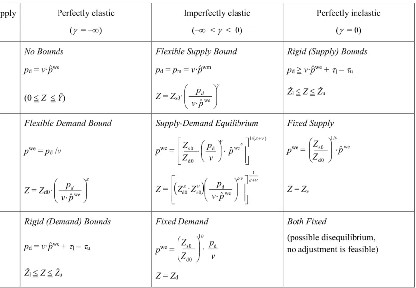
The main characteristics of the different export specifications are summarized in Table 1. The table contains all possible pairs of supply-demand elasticity situations. Some of them are not really relevant, since the export functions are only discussed here as part of more complicated (multisectoral) models.
It should be perhaps pointed out, and this is important from a computational point of view, that the usual demand-specified general equilibrium model can easily be modified to allow for alternative export specifications. If either ε or decreases beyond a certain limit, our
specification will reduce to the pure supply or demand case.
3 See, for example, Houthakker and Magee (1969), Hickman and Lau (1973), Sato (1977), Goldstein and Khan (1978), Stone (1979), Browne (1982).
Table 1. The choice of elasticity of export demand and supply and its effect on the model specification Supply
Demand
Perfectly elastic ( = –)
Imperfectly elastic (– < < 0)
Perfectly inelastic ( = 0)
Perfectly elastic ( = –, pwe = pwe)
No Bounds pd = v· pwe (0 Z Ȳ)
Flexible Supply Bound
pd = pm = v· pwm Z = Zs0·
pˆwe ν
pd
Rigid (Supply) Bounds pd v· pwe + l – u
Žl Z Žu
Imperfectly elastic (– < < 0)
Flexible Demand Bound pwe = pd /v
Z = Zd0·
pˆwe ν
pd
Supply-Demand Equilibrium pwe =
) /(
1 d we
0 d
0
s ˆ
p
v p Z Z
Z =
1
we s0 d
0
d · ˆ
p ν Z p Z
Fixed Supply pwe = we
/ 1
0 d
0
s pˆ
Z Z
Z = Zs
Perfectly inelastic ( = 0)
Rigid (Demand) Bounds
pd = v· pwe + l – u
Žl Z Žu
Fixed Demand pwe =
v p Z
Z 1/ d
0 d
0 s
Z = Zd
Both Fixed
(possible disequilibrium, no adjustment is feasible)
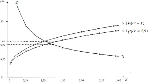
Figures 1 and 2, based on numerical simulations, summarize the main features of the alternative export specifications in geometrical form. Along the horizontal axis one can see the export volume (Z) in both cases. In Figure 1 the vertical axis represents the unit export price (pwe), whereas in Figure 2 the foreign currency equivalent of the domestic price (pd/v).
Figure 1. Export demand (D) and supply (S) as function of the export price (pwe)
Figure 2. Export demand (D), supply (S) and equilibrium (E) Figures 1 and 2, based on numerical simulations, summarize the main features of the alternative export specifications in geometrical form. Along the horizontal axis one can see the export volume (Z) in both cases. In Figure 1 the vertical axis represents the unit export price (pwe), whereas in Figure 2 the foreign currency equivalent of the domestic price (pd/v).
The figures illustrate the impact of a 10 percent change in pd/v on the volume of export in each case, which increased by 37, 23 and 13 percent in the supply, demand and equilibrium
specifications, respectively. The elasticities of supply and demand are -3 and -2, respectively, and therefore the export elasticity in the equilibrium specification will be -1,2.
6. EXPORT SUPPLY FUNCTION DERIVED FROM OPTIMIZING DECISION
The necessary conditions of optimal solution or equilibrium containing an export supply function as above could be derived from a programming model or on the bases of neoclassical economic theory, i.e., assuming profit maximizing behaviour, if the same product sold on the domestic and on the foreign market were less than perfect subsitutes, i.e., differentiated commodities.
This can be built into the model by means of a production function extended to joint production. In this function, on the one hand, a transformation (disaggregating) function, X(Cd, Z) = CAP shows what combinations of Cd and Z can be produced by distributing the given capacity CAP between the two sorts of output. The capacity (CAP) itself, on the other hand, provided by the available amount of production factors, say, labour (L) and capital (K), is expressed by a CAP = F(L, K) production (aggregating) function. Such a production
function will be thus defined as X(Cd, Z) = F(L, K). In our model the capacity is assumed to be fixed (Ȳ), therefore, the production function is reduces to equation X(Cd, Z) = Ȳ.
Changing the composition of Cd and Z, the factors of production have to be reallocated, and consequently, their productivity, that is the effective volume of the total capacity would fall, as a rule. This phenomenon can be represented by transformation functions. The most commonly used Constant Elasticity of Transformation (CET) function has the following linearly homogenous (homogenous of degree one) form:
X(Cd, Z) = (a·Cd + b·Z)1/,
where a and bare the usual share parameters, > 1 is the parameter determining < 0, the elasticity of transformation between the two types of products: = 1/(1 – ). This will be the price elasticity of export supply. This is why we use the same symbol here as in the case of the simple (econometrically estimated) export supply function.
At given pd and pe, i.e., the price of the product sold on domestic market and the price of its export converted to domestic currency, the profit maximizing producers will choose such a combination of Cd and Z, which maximizes their total revenue (pd·Cd + pe·Z) subject to the capacity constraint X(Cd, Z) = Ȳ. From the necessary conditions of that maximum one can derive convenient forms, which could be used in a general equilibrium model. For example, the following variables and equations:
– the unit (CET average) price of the composite product, X = X(Cd, Z):
pa = (pd·Cd + pe·Z)/X,
– re and se, the optimal ratio of export to domestic supply (Z/Cd) and to total production (Z/X):
re = re0·
e d
p
p , and se = se0·
e a
p p ,
– which implies the export supply functions of the following type:
Z = re·Cd = re0· ·
e d
p
p Cd and Z = se·Cd = se0· ·
e a
p p X.
Introducing the nonlinear transformation function into the programming model will produce similar effect as the export demand function: it will constrain the shift in the export volume.
Unlike in the case of the demand function, one can maintain the assumption of a small open economy, i.e., the export price is dictated by the world market (pwe). Change in the export volume will not bring about unexplainable change in the terms of trade and the assumption of optimising behaviour will not result in optimal tariff.
Assuming optimising behaviour will thus lead to the following programming problem:
NLP II The primal problem The Kuhn–Tucker complementary conditions
Cd, Cm, Z, M 0 pa, pm, v 0
(pa) X(Cd, Z) Ȳ pa·X/Cd 1 (L/Cd)
(pm) Cm M 0 pm 1 (L/Cm)
(v) pwm·M pwe·Z 0 pa·X/Z v· pwe (L/Z)
Cd + Cm max! pm v· pwm (L/M)
Assuming again that in the solution all variables become positive, all conditions, defined in the form of weak inequalities, will be fulfilled as equations. Using auxiliary variables pd and pe to denote the domestic price of the goods supplied on the domestic and the export markets, respectively, we get the following chain of equations:
pd = pa·X/Cd (= 1), pe = pa·X/Z (= v· pwe), pm = v· pwm (= 1).
By virtue of Euler’s theorem, one gets the following identities:
pd·Cd + pe·Z = pa·(X/Cd·Cd + X/Z·Z) = pa·Ȳ.
The necessary conditions of the optimal solution can be thus rewritten in the form of the following equation system,
GEM IV (1) X(Cd, Z) = Ȳ (5) pd = 1
(2) Cm M = 0 (6) pm = 1
(3a) pwm·M pwe·Z = 0 (7a) pe = v· pwe (4b) Z = se0· ·
e a
p
p Ȳ (8) pm = v· pwm
(9) pa = (pd·Cd + pe·Z)/Ȳ Compared to GEM II one can see that this equation system has nine variables instead of eight.
There are two new variables, pe and pa (the product price became differentiated and their average price became a new variable) and pwe has been dropped (the export price is no longer
variable). At the same time, the equation defining the average product price entered into the model. It should be noted that pa could be defined also as a CET dual function of pe and pa
alone, i.e., without using Cd, Z and Ȳ. Note also that the form of the export supply function matches the one used in GEM III, as long as the capacity, Ȳ is fixed, since se0·Ȳ suits Zs0. 7. INDIVIDUAL BOUNDS ON IMPORTS
A similar flexible bound approach can be used in case of the import as well, instead of individual rigid bounds. In our simple model it will be enough to constrain either the volume of export or import by individual bounds. In the case of import, the ratio of imported goods to domestic supply (rmd = Cm/Cd) is typically constrained. We introduce therefore only an upper (řu) and lower (řl) bound on the ratio of imported goods to domestic supply (rmd = Cm/Cd) into LP model III. Let us denote by lm and um the shadow-prices associated with the lower and upper constraint on import ratio, respectively. Modifying accordingly the LP problem one gets the following primal and dual problem.
LP III Primal problem Dual problem
Cd, Cm, Z, M 0 pd, pm, v, lm, um 0
(pd) Cd + Z Ȳ pd 1 – lm·řl + um·řu (Cd)
(pm) Cm M 0 pm 1 + lm – um (Cm)
(v) pwm·M pwe·Z 0 pd v· pwe (Z)
(lm, um) řl·Cd Cm řu·Cd pm v· pwm (M)
Cd + Cm max! pd·Ȳ min!
Observe that if the lower limit on imports is binding (neglecting degenerate solutions), we will have lm > 0, um = 0 and pd = 1 – lm·řl < 1, pm = 1 + lm > 1. If the upper limit is binding then lm = 0, um > 0 and pd = 1 + um·řu > 1, pm = 1 – um < 1. Otherwise pd = pm = 1. This means, that if pd > pm (the shadow-price of the commodity imported is smaller than that of the domestic), the volume of import will be as large as allowed for, and it will be the other way around, the import will be the minimum prescribed, if pd < pm.
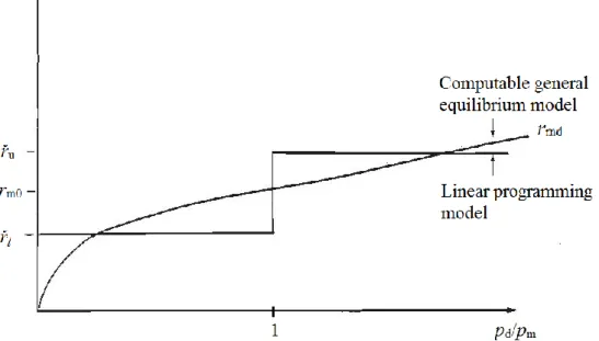
The import ratio can be defined, thus, by the following function (see its graph in Figure 3):
řl if pd/pm < 1 rmd = rm(pd, pm) = (řl, řu) if pd/pm = 1 řu if pd/pm > 1
Observe that the same import restriction could be achieved by modifying the C = Cd + Cm
objective function. One could introduce in its place a piecewise linear objective function with indifference curves as illustrated in Figure 4. That would in effect restrict the import ratio by the same lower (řl) and upper (řu) bounds as before. Such an objective function can be viewed as a piecewise linear welfare or utility function, whose indifference curves consist of three
different sections. Between the lines defined by Cm = řu·Cd and Cm = řl·Cd, i.e., when řl·Cd Cm řu·Cd, the two types of the commodity are perfect substitutes, beyond it they behave as perfect complements.
Figure 3. Smooth versus piecewise linear import ratio functions
Figure 4. Import restriction built into the objective function
In the computable general equilibrium (CGE) models, it is usually assumed (the so-called Armington assumption) that the domestic and the imported variety of the same commodity are less than perfect substitutes, represented by a Constant Elasticity of Substitution (CES) utility (use value aggregation) function of the following form:
C = C(Cd, Cm) = (d·Cd + m·Cm)1/,
where > –1 is the parameter determining > 0 the elasticity of substitution between the two types of commodity: = 1/(1 + ). The import ratio function (rmd) can be derived from maximizing the C(Cd, Cm) aggregation function subject to cost constraint pd·Cd + pm·Cm = 1.
The additional two constraints derived from the Lagrange function are as follows:
pd = C/Cd (L/Cm), pm = C/Cm (L/Cm)
From these necessary conditions one can derive the determination of the optimal ratio of the domestic and imported supply (Cm/Cd) in the form of a smooth function of their prices:
rmd =
d m
C
C = rm(pd, pm) = rm0·
m d
p p (see its curve in Figure 3).
The difference in the treatment of import restrictions between linear programming and computable equilibrium models can be seen again as the difference between using rigid or flexible individual bounds. The relative-price-dependent import ratio implies a flexible
individual bound on imports. The larger is the gap between the shadow-prices of the domestic and imported commodities the larger will be the deviation from the observed (or planned) import ratio (rm0).
Smooth import ratio functions could be incorporated into an otherwise linear model, as mentioned above, using a piecewise linearization technique.4 Thanks to availability of
efficient programs solving nonlinear programming or computable general equilibrium models, it is more advantageous to transform the model into a nonlinear form.
Suppose we have a linear programming model with fixed individual bounds on both exports and import ratios. If we want to replace the fixed individual bounds by flexible ones, as described earlier, one should replace the objective function with a smooth preference function reflecting import limitations and introduce an export demand function as before. These
changes yield the following nonlinear programming model.
NLP III The primal problem The Kuhn–Tucker complementary conditions
Cd, Cm, Z, M 0 pd, pm, v 0
(pd) Cd + Z Ȳ pd C/Cd (L/Cd)
(pm) Cm M 0 pm C/Cm (L/Cm)
(v) pwm·M pwe·Z 0 pd v· pwe (L/Z)
C(Cd, Cm) max! pm v· pwm (L/M)
4 See, for example, Ginsburgh and Waelbroeck (1981) again, who give examples showing how piecewise linear (nonlinear) relationships can be introduced into linear programming models and outline some applications.
If all variables are positive, which implies that all constraints are fulfilled in the form of equality, the necessary conditions of optimum can be reformulated into the form of the following system of simultaneous equations (containing Cd, Cm, Z, M, pd, pm, v as variables).
GEM V (1) Cd + Z = Ȳ (5) pd = v· pwe
(2) Cm M = 0 (6) pm = v· pwm
(3) pwm·M pwe·Z = 0 (7) pd·Cd + pm·Cm = 1 (4) Cm = rm0·
m d
p
p ·Cd
These are again the same as the necessary conditions of general equilibrium.
8. EQUILIBRIUM VERSUS OPTIMUM:OPTIMAL TARIFF REVISITED
It is worth taking a short detour and to show that by means of a slight modification of the NLP III model and making use of the parametric programming technique one can arrive at such a solution of the programming model, in which the necessary conditions of the optimal solution coincide with conditions if a perfect market equilibrium even in the case of downward sloping export demand function. The underlying idea is very simple. 5
We will simplify the description of the NLP model by assuming that all variables will be positive, thus all weak inequalities will be fulfilled as equations in the optimal solution. Since M will be equal to Cm, one can reduce the model by omitting variable M and dual variable pm
as well the corresponding complemetarity dual condition. Our programming problem will have only three variables and two constraints This will allow us to illustrate together and compare the optimal tariff solution (the “planners optimum”) and the perfect market equilibrium solution on Figures 5 and 6, making use of the Cd = Ȳ Z correspondence.
The modified model is as follows:
NLP IV The primal problem The Kuhn–Tucker conditions
Cd, Cm, Z 0 pd, pm, v 0
(pd) Cd + Z = Ȳ pd = 1 (L/Cd)
(v) pwm·Cm [/(1 +)]·pwe(Z)·Z = k v· pwm = 1 (L/Cm)
C(Cd, Cm) max! pd = v·pwe(Z) (L/Z)
The model which results in the optimal tariff solution has been modified in such a way that its dual conditions will satisfy the pricing requirements of perfect market equilibrium. This is achieved simply by multiplying the export term in the foreign currency constraint by factor
5 This idea was inspired by Lundgren (1982), who proposed such an algorithm for solving a special type of multisectoral equilibrium model, which incorporates non-smooth relationships.
/(1 +), the reciprocal of the optimal tariff term, in order to offset the "monopoly distortion"
effect in the Kuhn–Tucker conditions. This change, however, alters the meaning of the
foreign currency condition and this must be taken into account in the method of solution. This is achieved by varying the left-hand side (k) parametrically until the solution (Cm and Z, in particular) also satisfies the original current account, pwm·M pwe·Z = 0 condition.
Figure 5 sheds more light on the nature of the competitive equilibrium solution. The
horizontal axis represents primarily the value of Z. However, since the difference between Ȳ and Z yields Cd, whose value can be also represented along the horizontal axis. A vertical axis represents Cm in both cases As a result one can represent the indifference curves of C(Cd, Cm), the balance of payment condition, as well as the similar second constraint of the programming problem all on the same figure.
The curve from 0 to d = 0 represents the export-import combinations which fulfil the current account requirement, where d is the balance of current account. Notice that the only
difference between the latter and the second constraint in the programming model at k = 0 is that the export term is multiplied by the constant ε/(1 + ε), which is, by assumption, greater than 1. Therefore, the curve from 0 to k = 0 is steeper than the current account curve. The curve SȲ is the locus of the points, where the indifference curves of C(Cd, Cm) is tangent to the curve of 0 to k at various values of k.
Observe, that the optimal solution of the programming problem at k = 0 clearly does not meet the current account requirement. If, however, we change k parametrically then the optimal solution will lie on the curve SȲ. The competitive equilibrium is there, where this latter curve intersects the current account curve, the curve from 0 to d = 0.
From Figure 5 it is also clear, and it is even more apparent in Figure 6, that the pure
competitive equilibrium point cannot be the point of optimal solution at the same time. For, at the optimal solution point the indifference curve and the curve from 0 to k must be tangential to each other. In the competitive equilibrium case the current account curve and the curve from 0 to k*, which contains competitive equilibrium point, intersect each other. A small movement along the current account curve toward the origin would increase the value of the objective (welfare) function (see in Figure 6).
Observe the tangent line separating the indifference curve and to the transformed current account curve from 0 to k*at the equilibrium point is the consumers' budget line. This line passes through the origin (no foreign trade) as well, since the only source of income is the sale of domestic resources (pd·Ȳ). Observe, however, that this is not the case for the planners optimal solution, in which case part of the income is provided by the export tariffs.
9. SUMMING UP:NLP VERSUS CGEMODEL WITH FLEXIBLE BOUNDS
In the previous sections we have shown, case by case, how one can constrain the shift in export and import volume in macroeconomic models by means of flexible instead of rigid individual bounds as it is common in models of linear programming type. The basic idea was to use nonlinear relationships and thus assuming less than perfect substitutability between the
commodities and production factors used or produced jointly, borrowing the well-known techniques of microeconomics.