Method of Data Center Classifications
Krisztián Kósi
Óbuda University, Bécsi út 96/B, H-1034 Budapest, Hungary kosi.krisztian@phd.uni-obuda.hu
Abstract: This paper is about the Classification of big data centers, based on top500.org’s data. The classification begins with data weighting and Multidimensional Scaling.
Multidimensional Scaling produces 3D data. The clustering method, K-means, helps to classify the data. Nine different groups of data centers have been identified with appropriate parameters.
Keywords: Multidimensional Scaling; MDS; K-means; C-means; Clustering; Petri Net;
Classical Multidimensional Scaling; CMDS
1 Introduction
Two methods were used in this classification. The first is Multidimensional Scaling, also known as MDS. Multidimensional Scaling was developed originally by John W. Sammon Jr. in 1969 [1]. Many another variants have been developed;
the most common ones are Classical Multidimensional Scaling (CMDS), and Non-Metric Multidimensional Scaling. In this paper CMDS was used for problem solution. Classical Multidimensional Scaling allows many fine tuning and it is good enough for that method. Multidimensional Scaling can be used to reduce multidimensional problems into two or three dimensions [2].
Multidimensional Scaling has a wide spectrum of applications, such as Agricultural Economics [3], biology [4] Wireless Sensor Network Localization [5], Social Network Analysis [6], and Psychophysics [7].
One of the most popular clustering algorithms is K-means, also known as C- means. K-means has many implementations. Some of the most interesting implementations are High Parallel Implementation [8], Recovery for Burst-Mode Optical Receivers [9], and Clustering over a Peer-to-Peer Network [10].
2 The Main Algorithm
The algorithm consists of three main steps. (Fig. 1) The first major step is data preparation for MDS [13]. The second one is the execution of MDS, which creates a two or three dimensional point cloud. The last step is clustering with K-means.
The algorithm is very flexible; it has the possibility to change or tune its various parts.
Figure 1 The main algorithm
In the overall look, the algorithm is sequential, but some steps may have parallel implementation. The most convenient implementation can be done by the use of R. R is a free statistic environment [12], and most of the MDS methods and a lot of clustering algorithms are implemented in R. It can be used simply as a function call.
3 Data Preparation
The first step is the preparation part. This part is about putting the data into a starting matrix and creating a distance matrix from it. This part is one of the most flexible parts. There are possibilities for weighting the problems and determining which attributes are more significant than the others. For distance definition, a wide assortment of various norms is available.
The starting matrix must contain measurable values. Classical Multidimensional Scaling works just on numbers. In the matrix, the row index denotes the number of the appropriate element, while in the columns the attributes are numbered (Table 1).
The next step is optional. Weights can be applied to the starting matrix with the following tensor (1), where is the weight and represents the number of the appropriate attribute. This tensor recreates the matrix, which is more suitable for the problem. Expression (1) describes the square of the distance between elements i and j.
Table 1 Start Table
Attr. 1 Attr. 2 Attr. 3 Attr. n
1
2
3
4
5
m
[ ] [
]
[ ] (1)
CMDS needs a rectangular, symmetric distance matrix, the main diagonals of which are zeros. Because the distant matrix is symmetric, the upper part can be filled in with zeros too. Computing the distance matrix means getting the norms of the difference of elements (2). The results have to be placed into the distance matrix.
For this purpose, an arbitrary norm can be applied.
‖ ‖ (2)
[
]
(3)
4 Multidimensional Scaling
The Multidimensional Scaling part reduces the multidimensional problem into a two or three dimensional one, which can be visualized.
CMDS is satisfactory for this purpose because the distant matrix is rectangular and symmetric.
The first step is to choose a vector (4), where I is the dimension where the problem will be scaled.
Usually will be two or three dimensional.
(4)
The norm of the difference between the elements of has to be approximately equal to the distance (5).
‖ ‖ (5)
Vector has to be chosen to minimize the following expression (6).
∑ (‖ ‖ ) (6)
After the minimization, will represent the problem in the selected dimension.
The upper part of the matrix is not necessary in R. In the literature, various measures of goodness are applied for assessing the result of a fitting. The so called Shepard plot describes the distances versus the dissimilarities in a 2D diagram [13]. If the individual data fit well to the y=x line with little standard deviation, the fitting is good. If the points scatter too much around the line, the fitting is not too good. In the software package R that was applied for the calculations, the CMDS function used the best fitting algorithm, and no goodness measures were available as a default. For the purposes of this research, the default option was quite satisfactory.
The idea behind Multidimensional Scaling originally was the distance between two cities that is measurable with a ruler on the map. The main problem was how to recreate the map from the distance data. A popular example is flight paths between large cities in the USA.
5 Clustering
The clustering part is to decide which elements are in the same group. One of the most popular clustering methods is the K-means. The following Petri Net is about the base of the K-means clustering algorithm Fig. 5.
In an intuitive way, the clustering method creates groups around a set of points.
Each group has a center point. A point belongs to a particular group if it is closer to the center point of this group than to the center points of the other groups.
The points created by MDS in the selected dimension are denoted as (7).
(7)
Figure 5
K-means described by a Petri Net Each group has a center denoted by (8).
In the K-means algorithm, we need to know how many groups we have. It can be estimated from the figure of the finished Multidimensional Scaling.
(8)
Let us use the matrix of size for describing the grouping of the individual elements. Let if elements is in the group j, otherwise (10). Let be defined by the following expression (9).
∑ ∑ ‖ ‖ (9)
{
(10)
must be minimized under the following constraints: each element must belong to only one of the groups, i.e. for each j ∑ . Furthermore each element must belong to one of the groups.
The minimization of cannot be solved in closed form. There are many ways to solve this problem, but one of the good ways is to solve it with iteration.
Iteration steps:
0. Initialization: choose random centers.
a. choose optimal points to fixed centers.
b. choose optimal centers to fixed points.
Repeat ”a” and ”b” steps until convergence.
If the groups remain invariant, the algorithm can be stopped.
There are exact forms for the individual steps.
This minimization algorithm does not always work. However, in most of the practical cases it works perfectly.
Step ”a” can be computed with the following expression (11).
{ ‖ ‖
(11)
If a point can belong to more than one group according to (11), some arbitrary choice must be done.
Step ”b” can be computed with the following expression (12). is the number of points in the cluster (13).
∑ (12)
∑ (13)
6 The Particular Data under Consideration
The starting data is from top500.org [14]. The attributes chosen from the list that was released in November, 2011 are: Year, Total Cores, Accelerator Cores, Rmax, Rpeak, Efficiency, Processor Speed, and Core per Socket. Rmax and Rpeak are performance values from the LINPACK benchmark in TFlops. The Rmax is the maximal performance that LINPACK achieved; Rpeak is a theoretical peak value.
Due to the fact that the order of magnitudes of the original data in the above specified fields roughly corresponded to the significance of the appropriate attributes, no special weighting technique has been applied. That is, was used in the main diagonal elements of the matrix in (1).
For describing the distances at the starting point, Euclidean metrics was chosen because it is independent of the direction.
The second step is scaling the data. The distance has been transformed by the logarithm function (14). In the logarithmic function, the very short distances come loose, and the very far distances come closer (14). In this manner, more compact and distinguishable structures can be obtained.
(14)
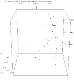
7 The Results by CMDS Using All Attributes
After applying the Multidimensional scaling for the all dataset, we obtained Fig. 6.
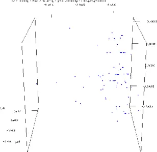
In Fig. 6 two well-defined big groups having internal fine structure can be revealed. To find the parameter according to which the whole set is split into these groups, one of the attributes can be neglected in MDS. This investigation can be done quite systematically. It was found that the attribute "Accelerator Cores"
caused this splitting. According to Fig. 7, by neglecting this attribute, only one big group can be obtained (of course, with internal fine structure).
Figure 6
CMDS with scaling
Figure 7
Without Accelerator Cores attribute, CMDS applied with scaling
8 Classification of the Fiber Structure
In the first group, the significant splitting attribute was Rmax (Fig. 8). Dropping two other attributes ("Rpeak" and "Total Cores") caused a less significant reduction in the structure (Figs. 9, 10).
The same method was applied for the investigation of the other seven main groups with the results as follows:
The second group’s main attribute is the Efficiency; the side attributes are Rmax and Rpeak.
The third group’s main attribute is the Efficiency too, but the side attribute is Processor Speed.
The fourth group’s main attribute is the Rpeak; the side attributes are Total Cores and Rmax.
The fifth group’s main attribute is the Year; the side attributes are Core per Socket, Processor speed, Efficiency.
The sixth group’s main attribute is the Processor speed, and the side attribute is Rmax.
The seventh group’s main attribute is the Total Cores, and the side attributes are Rmax and Rpeak
The eighth group’s main attribute is the Total Cores.
Figure 8 First group, Rmax
Figure 9 First group, Rpeak
Figure 10 First group, Total Cores
9 The Software Environment
R is a software environment for statistic computing [15], which is Open Source and free, available under GPL. The R is another implementation of S language and environment, which originally was developed by Bell Laboratories [15]. In these investigations, for this reason an implementation of R was used on a laptop with a Linux system. In this manner no extra programming activity was needed for the investigations. After specifying the initial matrix, the necessary computations were automatically executed, and appropriate figures were immediately displayed.
Conclusions
The combination of MDS and C-means clustering is a useful tool of classification for measurable multidimensional problems.
This method is very flexible. It can be fitted to real problems easily, just by fine- tuning the problem with weights, or by choosing other norms. The Clustering part is changeable. It is very easy to implement a short script in R and plot many variations. This helps to decide which modifications are the best.
This classification could help planning the computer systems of Data Centers. In future research, further attributes can be involved in the investigations. These attributes can be some service based system parameters, such as some kind of availability for software, hardware, and service. This could be service based planning, as well.
References
[1] John W. Sammon Jr., A Nonlinear Mapping for Data Structure Analysis IEEE Transactions On Computers, Vol. C-18, No. 5 (May 1969)
[2] Seung-Hee Bae, Jong Youl Choi, Judy Qiu, Geoffrey C. Fox, Dimension Reduction and Visualization of Large High-Dimensional Data via Interpolation HPDC’10, ACM 978-1-60558-942-8/10/06 (June 20-25, 2010)
[3] Douglas Barnett, Brain Blake, Bruce A. McCarl, Goal Programming via Multidimensional Scaling Applied to Senegalese Subsistence Farms American Journal of Agricultural Economics, Vol. 64, No. 4 (Nov. 1982) (pp. 720-727)
[4] Julia Handl, Douglas B. Kell, and Joshua Knowles, Multiobjective Optimization in Bioinformatics and Computational Biology IEEE/ACM
TRANSACTIONS ON COMPUTATIONAL BIOLOGY AND
BIOINFORMATICS, Vol. 4, No. 2 (APRIL-JUNE 2007)
[5] Frankie K. W. Chan and H. C. So, Efficient Weighted Multidimensional Scaling for Wireless Sensor Network Localization IEEE TRANSACTIONS ON SIGNAL PROCESSING, Vol. 57, No. 11 (NOVEMBER 2009)
[6] Purnamrita Sarkar, Andrew W. Moore, Dynamic Social Network Analysis using Latent Space Models SIGKDD Explorations, Vol. 7, No. 2
[7] James A. Ferwerda, Psychophysics 101 SIGGRAPH 2008 Courses Program (2008)
[8] Vance Faber, John Feo, Pak Chung Wong, Yousu Chen, A Highly Parallel Implementation of K-Means for Multithreaded ArchitectureHPC ’11 Proceedings of the 19th High Performance Computing Symposia (2011) [9] Tong Zhao, Arye Nehorai, Boaz Porat, K-Means Clustering-based Data
Detection and Symbol-Timing Recovery for Burst-Mode Optical Receiver IEEE TRANSACTIONS ON COMMUNICATIONS, Vol. 54, No. 8 (AUGUST 2006)
[10] Souptik Datta, Chris R. Giannella, and Hillol Kargupta, Approximate Distributed K-Means Clustering over a Peer-to-Peer Network IEEE TRANSACTIONS ON KNOWLEDGE AND DATA ENGINEERING, Vol. 21, No. 10 (OCTOBER 2009)
[11] Forrest W. Young, Multidimensional Scaling Kotz-Johnson (Ed.) Encyclopedia of Statistical Sciences, Vol. 5 (1985)
[12] http://www.r-project.org (2011 Dec.)
[13] R. Shepard, The Analysis of Proximities: Multidimensional Scaling with an Unknown Distance Function, I, II, Psyhometrika, 27, 219-246, 1962 [14] http://top500.org (2012 April)
[15] The R Development Core Team, R: A Language and Environment for Statistical Computing: Reference Index, ISBN 3-900051-07-0 (2011- 09- 30)