O R I G I N A L S T U D Y
The application of a combination of weighted least- squares and autoregressive methods in predictions of polar motion parameters
Fei Wu1•Kazhong Deng1•Guobin Chang1•Qianxin Wang1
Received: 7 May 2017 / Accepted: 5 March 2018 / Published online: 19 March 2018 ÓAkade´miai Kiado´ 2018
Abstract This study employs a combination of weighted least-squares extrapolation and an autoregressive model to produce medium-term predictions of polar motion (PM) parameters. The precisions of PM parameters extracted from earth orientation parameter (EOP) products are applied to determine the weight matrix. This study employs the EOP products released by the analysis center of the ‘International Global Navigation Satellite System Service and International Earth Rotation and Reference Systems Service’ needs to be modified to ‘International Global Navigation Satellite System Service (IGS) and International Earth Rotation and Reference Systems Service (IERS)’ as primary data. The polar motion parameters and their precisions are extracted from the EOP products to predict the changes in polar motion over spans of 1–360 days. Compared with the com- bination of least-squares and autoregressive model, this method shows considerable improvement in the prediction of PM parameters.
Keywords Earth orientation productsWeighted least-squaresAutoregressive modelPolar motion prediction
1 Introduction
Earth orientation parameters (EOPs) include the nutation and precession parameters, the polar motion parameters and the length of day (LOD). EOPs contain a wealth of geody- namics information and play a significant role in applications including the determination of high-precision satellite orbits, spacecraft tracking, laser measurements, and deep space exploration. These parameters are needed to achieve mutual conversion between celestial and terrestrial reference frames. Thanks to developments in modern measurement
& Kazhong Deng
kzdeng@cumt.edu.cn
1 School of Environment Science and Spatial Informatics, China University of Mining and Technology, Xuzhou 221116, China
https://doi.org/10.1007/s40328-018-0214-3
techniques, such as very long baseline interferometry (VLBI), satellite laser ranging (SLR), global navigation satellite system (GNSS), and doppler orbitography by radio-positioning integrated on satellite (DORIS) (Dow et al. 2005), increasingly accurate observations of EOPs promote advances in celestial dynamics.
Due to the complexity of the data processing involved, EOP products cannot be cal- culated in real time using the data obtained by modern earth observation technologies.
Thus, the parameters are usually provided after a delay of hours to days. However, for some practical applications, the EOPs must be acquired in advance. For example, in satellite navigation systems, only long-term predictions of EOPs can be used to achieve mutual conversion between the celestial and terrestrial reference frames when satellites enter the autonomous orbit mode. Therefore, a reliable and high precision prediction model is needed. However, EOPs are affected by many factors (Vo¨lgyesi 2006) that can be divided into two groups, specifically the effects of (1) different levels and periodic exci- tation sources and (2) high-frequency variations. These factors cause enormous challenges in the precise prediction of EOPs.
To check the accuracy of different methods of predicting EOPs, the Institute of Geodesy and Geophysics of the University of Vienna conducted two prediction competitions, the Earth Orientation Parameters Prediction Comparison Campaign (EOP PCC) in October 2005 (http://users.cbk.waw.pl/*kalma/EOP_PCC/) and the Earth Orientation Parameters Combination of Prediction Pilot Project (EOPCPPP) in October 2010 (http://eopcppp.cbk.
waw.pl). The purposes of these activities were to encourage scholars worldwide to utilize different methods to predict EOPs and to assess the forecasting accuracy and applicability of various prediction methods. The prediction methods can be divided into two categories, specifically single models (including both linear and nonlinear models) and combinations of multi models (Freedman et al.1994; Schuh et al.2002; Kosek et al.2004,2008; Xu 2012; Guo et al.2013; Xu and Zhou2015). One major conclusion that was reached as a result of these competitions is that no single prediction technique is suitable for all EOPs over their entire ranges of variation. The following two conclusions were also reached. (1) Least-squares extrapolation of harmonic models and autoregressive prediction (LS?AR), spectral analysis and LS extrapolation, and neural networks display relatively good per- formance in predicting PM. (2) Kalman filters, wavelet decomposition and auto-covariance prediction, and adaptive transformation of the atmospheric angular momentum (AAM) yield relatively high-quality results in predicting UT1-UTC and LOD (Kalarus et al.
2007,2010).
Many scholars have carried out studies on methods of predicting polar motion (Zhang 2012; Sun2013; Lei2016). Of these methods, LS?AR models represent a relatively stable type of model that is used to predict PM parameters; moreover, many scholars have made different improvements to this method (Sun and Xu2012; Xu et al.2012a,b; Yao et al. 2013). Note that the high calculation precision of the PM parameters is almost negligible compare with the prediction accuracy; thus, the effects of model error on the predictions should be emphasized. Therefore, how to address the residuals that result from fitting LS models to data has been examined by different scholars. Differential method processing LS?AR models are used mainly in short-term forecasts (Yan and Yao2012), whereas WLS?AR models are employed in medium-and-long-term predictions of PM parameters. The main principle used by previous studies to construct the weight matrix is that relatively high weights are assigned when the predicted values lie close to the data;
although this practice effectively improves the prediction accuracy, it depends consider- ably on the experience of the operator (Sun and Xu 2012). Therefore, in this paper, we propose employing the calculation precision of the PM parameters extracted from EOP
products as weighting factors to determine the weight matrices of the vectors of obser- vation used in the least-squares extrapolation model. In this study, the fitting parameters of the weighted least-squares model are first calculated; the AR model parameters are then determined from the residuals; and finally, the extrapolated values obtained from the WLS and AR models are combined to obtain the final predictions. Having extracted PM parameters and their precisions from the data products published by the analysis centres of the IGS and the IERS, which are taken to represent basic data, this study predicts medium- term changes in PM and compares them with the results predicted by the LS?AR model to verify the feasibility of the method presented here.
2 Methods
2.1 Weighted least-squares model
The method is based on LS?AR. An introduction to the construction of and the calcu- lations performed by the model is first presented. Existing studies have shown that the major trends of the PM contain a linear term and periodic terms, including the Chandler wobble and the annual and semi-annual terms (Sun2013). The fitting equation of the LS model can be expressed as:
Xð Þ ¼t a0þa1tþa2cos 2pt T1
þa3sin 2pt T1
þa4cos 2pt T2
þa5sin 2pt T2
þa6cos 2pt T3
þa7sin 2pt T3
ð1Þ where X(t) is the PM at timet;tis the UTC time (in years);a0;a1;a2;a3;a4;a5;a6;a7need to be estimated;T1;T2;T3are the periods of the semi-annual, annual and Chandler wobble terms, respectively. In this paper, T1¼0:5a;T2¼1aandT3¼1:183a. Estimates of the model parameters can be calculated using formula (2):
a¼ATPA1
ATPL ð2Þ
a¼½a0 a1 a2 a3 a4 a5 a6 a7T ð3Þ L¼½X tð Þ1 X tð Þ 2 X tð Þn T ð4Þ
A¼
1 t1 cos 2pt1
T1
sin 2pt1
T1
cos 2pt1
T2
sin 2pt1
T2
cos 2pt1
T3
sin 2pt1
T3
...
... ...
...
...
...
...
... 1 tn cos 2ptn
T1
sin 2pt1
T1
cos 2ptn
T2
sin 2ptn
T2
cos 2ptn
T3
sin 2ptn
T3
2
66 66 64
3 77 77 75
ð5Þ whereais the vector of estimated parameter; Ais a coefficient matrix;Lis a vector of observation; andPis the weight matrix, which is a diagonal matrix. The residuals are then processed using an AR model.
2.2 Determination of the weight matrix
The key feature of the WLS method is that it incorporates a weight matrix into the estimation of parameters based on LS models. An appropriate weighting method effec- tively improves the precision of the model parameters, thus resulting in a more stable base sequence for the AR model. In the actual process of surveying adjustment, using the calculated precision of the parameters as the posterior factor is a commonly weighting method. Therefore, this paper extracts the precision of PM parameters from the EOP products released by different analysis centers for use as a variance factor in building the weight matrix. The weight matrix is expressed as follows:
Pw¼ r20
r21;w 0 0 0 0 r20
r22;w 0 0 ...
... .. .
...
0 0 0 r20
r2n;w 2
66 66 66 66 66 4
3 77 77 77 77 77 5
ð6Þ
wherewdenotes the polar motion (PMX, PMY);nis the length of the basic data; the unit weight variance r20 is assigned a value of 1; and r2n;w represents the variances of the calculated PM parameters on thenth day.
2.3 AR model
An AR model describes the relationship among the variables of a random series
ztðt¼1;2;. . .NÞ, which can be expressed as follows:
zt¼Xp
i¼1
uiztiþet ð7Þ
where u1;u2;. . .up are autoregressive coefficients obtained using the least squares method;pis the order of the model; anderepresents zero-mean white noise. In this paper, the AR model is constructed by the fitting residuals of the WLS model.
A key step in applying AR model is determining the orderp. Three main methods of estimating the orders of AR model exist. Specifically, these rules are the final prediction error (FPE) criterion, the akaike information criterion (AIC), and the criterion autore- gressive transfer (CAT). In practice, these three methods are virtually equivalent to each other. The FPE criterion is adopted to determine the order of AR model.
FPEð Þ ¼p ðNþpÞ Np
ð ÞPp ð8Þ
where
Pp¼ 1 Np
XN
t¼pþ1
ztXp
j¼1
ujztj
!2
ð9Þ
Here p¼1;2;. . .N, andPp is the residual mean squared deviation of the model fitting sequence in AR(p). When FPE (p) reaches its minimum value, p is taken to represent the order of the best model.
2.4 Prediction error estimates
The mean absolute error (MAE) is an indicator of prediction accuracy. It is calculated as:
MAEi¼1 n
Xn
j¼1
SijOij
ð10Þ
whereiis the prediction interval;Sij;Oijare the predicted and released values, respectively, on day j; andnis the number of predictions used to calculate the statistics.
3 Examples and analysis
The products released by IGS and IERS contain the values and precision of PM param- eters, and the time interval used in the products is 1 day. However, the EOP products released by the IGS Analysis Centre are determined using GNSS technology, whereas those of the IERS Analysis Centre are calculated using multiple technologies (such as GNSS, VLBI, SLR, and DORIS); the precisions of the PM parameters are not the same. In this study, the EOP products released by IGS and IERS are used as basic experimental data to predict the medium-term PM and to verify the effectiveness of the method proposed. As recent studies have shown (Sun et al. 2015), the highest accuracies are obtained in pre- dictions using of the LS?AR models when an input sequence of 10 years is used.
Therefore, this thesis takes 10 years as an elementary sequence to predict PM using an interval of 1 day and a span of 1–360 days.
3.1 Experiments based on products released by IGS
The values and the precisions derived from the PM parameters products issued by IGS (ftp://cddis.gsfc.nasa.gov/pub/gps/products/), which extend from January 1, 2002 to December 31, 2011, are employed to construct the prediction model and build the weight matrix. For each prediction (1–360 days), 600 and 1000 experiments are performed using the LS?AR and WLS?AR methods. The predictions extend from January 1, 2012 to August 18, 2014 and January 1, 2012 to September 22, 2015, and the sampling interval is 1 day. Tables1and2list the MAE values for the different prediction intervals, and these values are shown graphically in Figs.1and2.
Table 1 Statistical accuracy results in 600 IGS forecasts
MAE PMX (mas) PMY (mas)
Prediction day
LS?AR WLS?AR Accuracy improvement (%)
LS?AR WLS?AR Accuracy improvement (%)
1 0.216 0.215 0.074 0.106 0.106 0
5 1.484 1.480 0.23 0.665 0.660 0.739
10 2.831 2.793 1.353 1.244 1.226 1.51
30 8.210 8.024 2.26 3.875 3.613 6.765
60 15.886 15.106 4.907 8.114 7.022 13.467
100 23.285 20.704 11.083 14.159 10.262 27.525
120 27.145 22.273 17.95 16.218 11.193 30.986
150 31.700 24.281 23.405 17.826 12.486 29.957
200 33.499 25.094 25.092 15.553 11.851 23.803
250 30.509 23.914 21.616 13.475 9.726 27.819
300 30.179 25.690 14.874 15.579 10.894 30.069
360 36.631 25.753 29.697 18.685 13.376 28.413
Table 2 Statistical of accuracy results in 1000 IGS forecasts
MAE PMX (mas) PMY (mas)
Prediction day
LS?AR WLS?AR Accuracy improvement (%)
LS?AR WLS?AR Accuracy improvement (%)
1 0.212 0.211 0.308 0.175 0.174 0.06
5 1.482 1.457 1.695 1.092 1.081 0.978
10 2.831 2.720 3.913 2.056 2.024 1.567
30 8.380 7.818 6.709 6.255 5.875 6.072
60 16.666 14.619 12.279 13.667 11.713 14.295
100 25.904 20.023 22.702 24.593 18.373 25.289
120 29.763 21.616 27.372 28.483 20.576 27.758
150 33.988 23.419 31.097 32.161 22.873 28.88
200 35.434 23.472 33.759 30.309 21.760 28.208
250 34.594 23.404 32.347 28.380 20.871 26.459
300 35.652 27.121 23.928 33.023 24.328 26.33
360 41.881 29.845 28.739 39.246 28.954 26.224
Fig. 1 MAE values calculated for 600 IGS forecasts over different intervals
Fig. 2 MAE values calculated for 1000 IGS forecasts over different intervals
3.2 Experiments based on products released by IERS
As another example, this study chooses the values and the precision of PM parameters issued by IERS 08 C04 EOP product (ftp://ftp.iers.org/products/eop/long-term/c04_08/
iau2000/), which extends from January 1, 2002 to December 31, 2011. These data are used to construct the prediction model and build the weight matrix. 600 and 1000 experiments are performed using the LS?AR and WLS?AR methods for each pre- diction (1–360 days), and the sampling interval is uniformly 1 day. The prediction dates are the same as the previous two experiments. The results are presented in Tables3,4 and Figs.3,4.
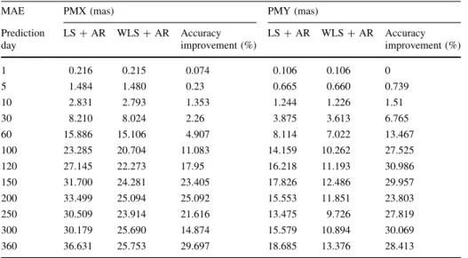
Table 3 Statistical of accuracy results in 600 IERS forecasts
MAE PMX (mas) PMY (mas)
Prediction day
LS?AR WLS?AR Accuracy improvement (%)
LS?AR WLS?AR Accuracy improvement (%)
1 0.224 0.223 0.23 0.108 0.108 0
5 1.492 1.479 0.88 0.662 0.654 1.182
10 2.895 2.836 2.018 1.237 1.213 1.974
30 8.785 8.190 6.77 3.873 3.540 8.587
60 17.603 15.323 12.95 8.143 6.996 14.091
100 25.168 20.725 17.653 14.207 11.114 21.774
120 28.619 21.680 24.246 16.265 12.706 21.879
150 33.230 24.343 26.744 17.840 13.974 21.673
200 36.156 24.995 30.869 15.459 12.271 20.623
250 33.790 24.508 27.468 13.287 9.564 28.018
300 32.471 25.898 20.242 15.427 11.918 22.747
360 37.064 26.997 27.161 18.691 15.557 16.765
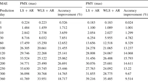
Table 4 Statistical of accuracy results for 1000 IERS forecasts
MAE PMX (mas) PMY (mas)
Prediction day
LS?AR WLS?AR Accuracy improvement (%)
LS?AR WLS?AR Accuracy improvement (%)
1 0.224 0.223 0.526 0.183 0.183 0.024
5 1.484 1.459 1.712 1.100 1.089 1.001
10 2.842 2.738 3.659 2.054 2.027 1.299
30 8.716 8.032 7.851 6.254 5.955 4.782
60 17.459 15.250 12.652 13.656 12.518 8.329
100 26.305 20.661 21.455 24.278 21.065 13.237
120 29.746 22.268 25.141 28.008 24.067 14.068
150 33.524 25.122 25.062 31.456 26.488 15.793
200 34.771 25.490 26.691 30.076 25.681 14.611
250 33.630 25.745 23.446 27.763 24.092 13.22
300 36.098 30.768 14.765 31.855 28.775 9.67
360 41.769 33.951 18.717 39.216 35.485 9.514
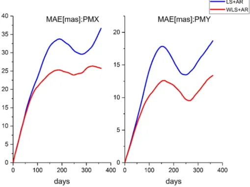
Fig. 3 MAE values calculated in 600 IERS forecasts
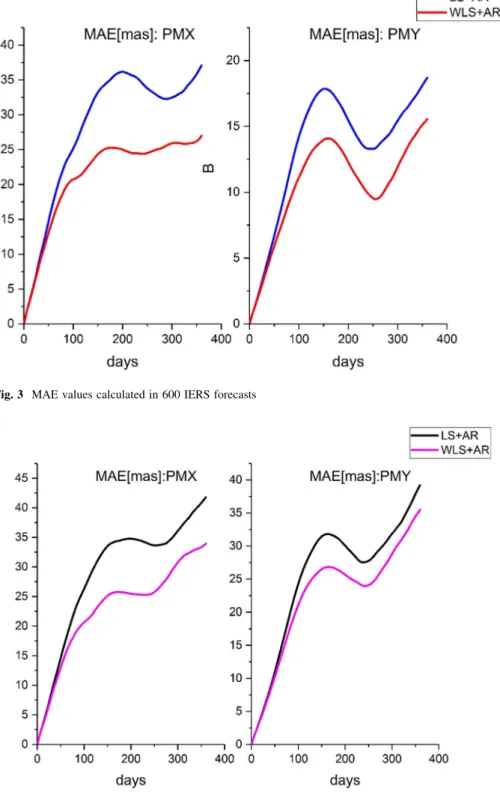
Fig. 4 MAE values calculated for 1000 IERS forecasts
The above results indicate that the prediction accuracy of the WLS?AR model shows improvement at different levels in both the PMX and PMY directions. The improvements in the forecasting accuracy for short-term predictions (1–30 days in the future) are not obvious; the maximum improvement in the polar motion parameters in the PMX direction is less than 8.19%, whereas that in the PMY direction is within 8.587%. However, when the prediction span exceeds 30 days, the accuracy of the prediction displays clear improvements. For the group of 600 experiments, the prediction accuracy in the PMX direction calculated using the IGS and IERS data increases by an average of 16.09 and 21.43%, whereas that in the PMY direction using the IGS and IERS data increases by 23.64 and 19.19%, respectively. In the group of 1000 experiments, the prediction accuracy in the PMX direction calculated using the IGS and IERS data increases by an average of 24.14 and 19.04%, whereas that in the PMY direction using the IGS and IERS data increases by 22.94 and 11.07%, respectively. Compared with the LS?AR model, the WLS?AR model generally better in predicting polar motion parameters and yields more accurate medium-term forecasts.
4 Conclusion
This paper proposes a method of producing medium-term predictions of polar motion parameters using a WLS?AR model. In this method, the calculation precision of the PM parameters is employed to produce weighting factors to build the weight matrix of the vector of observations in the least-squares extrapolation model. More accurate parameters and extrapolated values of the LS model while and more stable residuals to form and calculate the AR model can be obtained using this method. The EOP products released by the analysis center of IGS and IERS are used as the basic data to predict the polar motion parameters in groups of 600 and 1000 experiments with a 1-day prediction interval and a span of 360 days. The results of the experiments show that, compared with the LS?AR model, the WLS?AR model proposed in this paper effectively improves the accuracy with which polar motion parameters can be predicted.
Acknowledgements The work is supported by the Ordinary University Graduate Student Research Inno- vation Project of Jiangsu Province (KYLX16_0541), National Natural Science Foundation of China (41774005), National Natural Science Foundation of China (41404033), Open research fund projects of the state key laboratory (SKLGIE2014-Z-1-1) and Project on Basic Research of The National Department of Science and Technology (2015FY310200). We thank the IERS and IIGS for providing the EOPs products.
References
Dow JM, Gurtner W, Schlu¨ter W (2005) The IGGOS viewed from the space geodetic services. J Geodyn 40(4):375–386
Freedman AP, Steppe JA, Dickey JO, Eubanks TM, Sung LY (1994) The short-term prediction of universal time and length of day using atmospheric angular momentum. J Geophys Res Solid Earth 99(B4):6981–6996
Guo JY, Li YB, Dai CL, Shum CK (2013) A technique to improve the accuracy of earth orientation prediction algorithms based on least squares extrapolation. J Geodyn 70(10):36–48
Kalarus M, Kosek W, Schuh H (2007) Current results of the earth orientation parameters prediction comparison campaign. Proc Journe´es 84(10):587–596
Kalarus M, Schuh H, Kosek W, Akyilmaz O, Bizouard C, Gambis D et al (2010) Achievements of the earth orientation parameters prediction comparison campaign. J Geodesy 84(10):587–596
Kosek W, McCarthy DD, Johnson TJ, Kalarus M (2004) Comparison of polar motion prediction results supplied by the IERS Sub-bureau for Rapid Service and Predictions and results of other prediction methods. In: Finkelstein A, Capitaine N (eds) Proc. Journe´es 2003 Syste`mes de Re´fe´rence Spatio- Temporels, pp 164–169
Kosek W, Kalarus M, Niedzielski T (2008) Forecasting of the earth orientation parameters comparison of different algorithms. Nagoya J Med Sci 69(3–4):133–137
Lei Y (2016) Study on method for high accuracy prediction of earth rotation parameters. Chinese Academy of Sciences, Beijing
Schuh H, Ulrich M, Egger D, Mu¨ller J, Schwegmann W (2002a) Prediction of earth orientation parameters by artificial neural networks. J Geodesy 76(5):247–258
Sun Z (2013) Research on the theories and algorithms of earth rotation parameters prediction. Chang’an University, Xi’an
Sun Z, Xu T (2012) Prediction of earth rotation parameters based on improved weighted least squares and autoregressive model. Geodesy Geodyn 3(3):57–64
Sun Z, Xu T, He B, Ren G (2015) Prediction and analysis of Chinese earth rotation parameters based on robust least-squares and autoregressive model. In: China satellite navigation conference (CSNC) 2015 proceedings: vol II. Springer, Berlin, Heidelberg, pp 477–486
Vo¨lgyesi L (2006) Physical backgrounds of Earth’s rotation, revision of the terminology. Acta Geod Geophys Hung 41(1):31–44
Xu XQ (2012) Researches on high accuracy prediction methods of earth orientation parameters. University of Chinese Academy of Sciences, Beijing
Xu XQ, Zhou YH (2015) EOP prediction using least square fitting and autoregressive filter over optimized data intervals. Adv Space Res 56(10):2248–2253
Xu XQ, Zotov L, Zhou YH (2012a) Combined prediction of earth orientation parameters. In: China satellite navigation conference (CSNC) 2012 proceedings lecture notes in electrical engineering, 2012, vol 160, Part 2, pp 361–369.https://doi.org/10.1007/978-3-642-29175-3_32
Xu XQ, Zhou YH, Liao XH (2012b) Short-term earth orientation parameters predictions by combination of the least-squares, ar model and Kalman filter. J Geodyn 62(1016):83–86
Yan F, Yao Y (2012) Short-term prediction methods and realization of earth rotation parameters. J Geod Geodyn 32(4):71–75
Yao YB, Yue SQ, Chen P (2013) A new LS?AR model with additional error correction for polar motion forecast. Sci China Earth Sci 56(5):818–828
Zhang H (2012) Researches on the prediction theories and algorithms of polar motion of earth orientation parameters. Central South University, Changsha