Operations Research Letters

(1)

Contents lists available atScienceDirect

Operations Research Letters

journal homepage:www.elsevier.com/locate/orl

Binary integer modeling of the traffic flow optimization problem, in the case of an autonomous transportation system

Gábor Pauer

^∗

, Árpád Török

Budapest University of Technology and Economics, Department of Automotive Technologies, Faculty of Transportation Engineering and Vehicle Engineering, Műegyetem rkp. 3, 1111 Budapest, Hungary

a r t i c l e i n f o

Article history:

Received 8 July 2020

Received in revised form 2 December 2020 Accepted 3 December 2020

Available online 8 December 2020 Keywords:

Traffic

Cooperative traffic management Autonomous vehicle control Binary integer modeling

a b s t r a c t

Our research aimed to optimize the transportation processes through the binary integer modeling of cooperative vehicle control by linking the dynamic traffic assignment approach and controlling the autonomous transport system. Our paper’s main contribution is a model transforming the optimal vehicle control problem into binary integer formulation, optimizing transport processes at the system level, and representing safety and dynamics related constraints on the vehicle level. Two small numerical case studies have illustrated the applicability and effectiveness of the model.

1. Introduction and literature review

The growing number of highly automated vehicles on our roads will make it possible to control our transportation systems more efficiently [25,30]. However, we need to keep in mind that the real-time control of many agents can cause a relevant challenge for the traffic management system, even in the case of serious computing capacities [38]. This consideration made us develop a solution that can improve the efficiency of the traffic management process [21]. To identify the relevant research orientations, we reviewed the related works in traffic assignment and network capacity utilization [15].

As we expected, there is extensive literature in traffic assignment and network capacity utilization, based on various approaches. Peeta and Ziliaskopoulos [22] published a compre- hensive review of various dynamic traffic assignment models in their study. These models aim to identify a group of alternative routes between origins and destinations. One of the most commonly used traffic flow models is the cell transmission model (CTM) developed by Daganzo [8,9]. The fundamental diagram of traffic flow and density is assumed to be a piecewise linear function. Lo and Szeto [19,27] developed a cell-based dynamic traffic assignment formulation that follows the ideal dynamic user optimal principle. Waller and Ziliaskopoulos [33] efficiently solved the dynamic user optimal problem applying the CTM approach. The link transmission model (LTM) was developed by

∗ Corresponding author.

E-mail addresses: pgabor90@gmail.com(G. Pauer), arpad.torok@auto.bme.hu(Á. Török).

Yperman [34], addressing the limitations of CTM arising from its uniform cell-based discretization structure. Node models are also available for macroscopic simulation [28].

In real-life, the traffic distribution is based on road users’ decisions, influenced by external parameters (e.g., price, safety, con- gestions) as modeled in many research studies. A dual-time-scale formulation of dynamic user equilibrium (DUE) with demand evolution has been presented in the paper by Friesz, Kim, Kwon, and Rigdon [11]. They assumed that drivers adapt their mobility demands based on their congestion experiences of previous days.

Zhang and Waller [35] developed a heuristic model representing the interrelation of decision-makers and road users, suggesting a new framework for the transportation network design problem.

The research paper [12] pointed out that commuters decide the preferred mode that minimizes their total travel cost, while tran- sit agencies decide the operation time periods. These researches provided valuable results, but in light of technology advances, the role of users’ decisions may change significantly. With the spread of more and more effective information systems (e.g., traffic de- pendent, real-time navigation), route choice related processes of the road users can be influenced to become more rational. Thus, more efficient traffic management could be achieved [4,32].

With the growing penetration of autonomous vehicles (AVs), the proportion of random user decisions can be reduced. AVs have a high degree of control, which allows the transport system to respond to instantaneous situations cooperatively with high efficiency and flexibility [18]. Therefore, autonomous transportation has great potentials in increasing system efficiency, especially where the road resources are limited [24]. The research [5] highlights that AVs can intensify mode shifts and can

https://doi.org/10.1016/j.orl.2020.12.004

(2)

G. Pauer and Á. Török Operations Research Letters 49 (2021) 136–143

result in additional driven vehicle kilometers. This also shows the importance of efficient traffic and vehicle management that can increase efficiency in terms of energy and infrastructure utilization, resulting in less travel time and environmental pol- lution [16,29]. Based on these studies, it seems reasonable that new model development and optimization processes should focus on the representation of connected and automated transportation systems.

Numerous studies were carried out in the field of microscopic traffic management, aiming to optimize processes or parameters related to the transportation of AVs (such as path tracking control strategies [1], or design of lane-keeping algorithm [31]). From a macroscopic point of view, the paper of Hult et al. [14] highlights the main challenges of coordinating an autonomous transport system (a set of AVs) at the network level: the coordination problem can be defined as a constrained optimal control problem (OCP), where a performance criterion is optimized with respect to the vehicles’ control input trajectories, subject to safety (e.g., no collisions occur) and feasibility (e.g., destinations are reached eventually) requirements. Following the findings of the article by Hult et al. we can conclude that studies aimed at optimizing the management of AVs use (i) rule-based and (ii) optimization-based solutions [14].

Rule-based solutions implement a set of rules that specifies the communication between the elements of the transport system and the potential responses to the actions of other road users.

It is generally assumed that individual vehicles are capable of providing safe transport at the local level (e.g., they keep the lane, avoid rear-end collisions). At the same time, multipath conflicts (e.g., at an intersection) are solved by a central coordination manager that performs interventions based on dynamic data of vehicles [14]. The rule-based concept is adapted in the paper of Kowshik, Caveney and Kumar [17] through a hybrid architecture, where an infinite horizon contingency plan of each vehicle, as well as dynamically changing partial-order relation between cars were determined, and also centralized management was involved in coordinating intersection traffic flows. A reservation-based system was elaborated in the paper of Dresner and Stone [10], where cars request and receive time slots from the intersection during which they may pass. The system proved to be efficient but worked with serious restrictions (e.g., inability of vehicles to turn or change velocity in the intersection). A spatio-temporal technique was proposed by the article of Azimi, Bhatia, Rajkumar, and Mudalige [2], to manage the safe and efficient passage of autonomous vehicles through intersections, aiming to maximize capacity utilization, enforcing the synchronized arrival of AVs to the intersection. A new method for controlling the traffic at isolated intersections, proposing the control policy through structural analysis, was developed [20]. The main advantages of rule-based solutions are the distribution of computation and the economical use of communication resources. The method may outperform the current regulatory mechanism. However, they only focus on solving a partial problem (e.g., crossing of vehicles at an intersection) of the transport event chain. They cannot guarantee to reach the objective and meet the constraints of OCP. Therefore they most likely underutilize the potential of automated vehicles in coordination scenarios [14].

In the case of optimization-based solutions, the coordination problem is transformed into a mathematical program that can be solved with different algorithms and methods [23]. The optimization-based models’ main contribution is the possibil- ity to take different objective functions, dynamics, and physical constraints into account during the design process. With this, the system outputs can continuously be controlled and adjusted during operation. However, as a consequence, the computational complexity increases and grows exponentially with the number of possible conflict relationships among the vehicles [14].

Numerous optimization-based studies aimed the cooperative coordination of AVs at intersections [6,7,13]. The purpose of these methods is to determine control actions for the system agents (such as vehicles or other road users) in the intersections so that the transport system’s safety does not decrease (avoiding any collisions or conflicts). These papers’ contributions are mainly such reformulations, approximations, and heuristics that aim to reduce computational complexity. In the control problem, the vehicles are characterized by their position and its’ derivatives (velocity, acceleration). Optimization objectives are nonlinear, derived by the combination of vehicles’ states and control inputs. The vehicle navigation task was described as a constrained optimal control problem in the paper [26]. The constraints were derived from the traversable regions of the environment. This study focused on the design problem of the optimal vehicle trajectories aiming to minimize the risk level based on the vehicles’ current states and driver inputs. The model-based predictive traffic control for intelligent vehicles elaborated in [3] aimed to manage the lane allocations and speed limits in complex vehicle platooning processes. The model aimed to minimize the total time of vehicles spent in the network by solving the described mixed-integer optimization problem.

Based on the reviewed literature, we can conclude that the reduction of complexity is still a considerably relevant issue in the field of controlling autonomous transportations systems. On the one hand, this could allow us to extend the controlled system by increasing the number of controlled vehicles, the time, or the system’s spatial dimensions. On the other hand, the reduction of computational complexity could lead to moving system characteristics closer to real-time process control requirements.

Following this, the paper’s main aim is to develop a novel model architecture that enables us to represent the optimization problem of autonomous transportation processes in a binary integer system. The most important challenge of this development orientation is the consistent representation of velocity and acceleration since these factors are usually represented in nonlinear way.

2. Contributions of the paper

As presented above, yet the research of dynamic traffic assignment and control of autonomous transport is commonly treated separately, although clear linkage exists between the two processes. Using a novel approach, Zhu and Ukkusuri [37] developed a linear programming formulation assuming a connected vehicle environment, aiming to achieve both a system optimum based dynamic traffic assignment and autonomous intersection control. As a starting point, they used the lane-based traffic flow model from [34] and [36], introducing a complementarity constraint to ensure conflict-free traffic flows at intersections. Since the determined optimization problem was nonlinear and had a bi-level structure where it is hard to obtain an exact optimal solution, it has been transformed into a linear programming problem by relaxing the nonlinear constraints with linear inequalities and equations. The developed model achieved promising results based on three numerical case studies, demonstrating the benefit of its application in dynamic traffic assignment [37].

Although this study represented significant new results in linking AV control tasks and network-level traffic optimization, the authors primarily focused on the traffic assignment approach.

The road network was represented by a lane-based approach. Zhu and Ukkusuri [37] aimed to assign traffic volumes to the network components and minimize the total travel time by using lane occupancy as a system variable. Accordingly, the optimization task was to determine traffic flows without taking into account vehicle dynamics.

With a similar objective but based on a different approach, our study focuses on the network-level optimization of traffic

(3)

demand management through the binary integer modeling of cooperative vehicle control. In accordance with this, the variable of our model is the current position of the vehicles. The goal of optimization is to control vehicles on the network by:

• satisfying travel demands between the defined origin and destination zones (OD) while minimizing the traffic load of the network,

• assuring traffic safety at a local level (e.g., keeping the lane, avoiding rear-end collisions), and also at intersections,

• taking into account speed and acceleration/deceleration limits of vehicles to ensure realistic traffic maneuvers.

The developed model considers possible control interventions at the vehicle level. The control problem has been reformulated in a discrete-time domain by representing the system’s dynamic characteristics in a discrete form [14]. Time-space has been dis- cretized into time steps, where a finite time optimal control problem is solved at every step of the model. The road network has been partitioned into sufficiently small locations based on the size of passenger vehicles (unlike in the case of traditional cell- based transmission models (CTM) where the length of the cell is chosen such that it is equal to the distance traveled by free-flow traffic in one evaluation time step).

The advantage of the above considerations is that the position of vehicles can be accurately determined and controlled on the network at each model time step, therefore:

• traffic safety can be ensured (e.g., avoiding collisions on routes and at intersections),

• unlike in traditional CTM models, lanes can be considered, and lane management can be realized,

• due to the nature of the management process, capacity constraints of the road network elements are automatically taken into account.

However, it should be noted that such detailed partitioning of the network is a complex task, and the increase in the number of examined time steps and locations significantly increases the computational demand for control. The major weakness of the optimization-based AV control schemes is the complexity of the formulated problem due to the special requirements of the management processes [14]. The problem is mainly described in a nonlinear, non-convex, and difficultly-tractable form, where it is hard to obtain an exact optimal solution [37].

Our paper’s novel contribution is the development of a 0–1 integer programming formulation of the optimal control problem, realizing individual control of AVs with respect to the constraints arising from the considered safety and vehicle dynamics parameters, and thus optimizing traffic assignment at the system level.

Authors assume that all vehicles in the investigated transport system are fully autonomous and can be ideally controlled. As- suming theoretically ideal circumstances, we consider that the communication network is fully connected during the time period without any problems (such as delays, interference) in the communication process.

3. Presentation of the elaborated model

The developed model implements network-level optimization of traffic assignment through the cooperative control of autonomous vehicles, in a binary integer programming approach.

The process aims to satisfy the emerging travel demands in a way that minimizes the load of the network and assures safe transport.

3.1. Partition of the road network

The proper operation of the optimization model requires the road network to be partitioned into sufficiently small locations.

As the length of the locations determines the distance between vehicles, the size of them must be determined in a way to provide both safe and efficient transport (only one vehicle can be in one location at a time). Each location is directed. This kind of network representation allows the modeler to describe different types of lanes and intersections, as well as to avoid collisions by controlling the vehicles per location.

3.2. Defining the model variable and initial data

The binary decision variable of the model is indicated byxk,^j,ⁱ. where,

k– is the index of the represented vehicles (k=1. . .m), j– is the index of the considered time steps (j=1. . .t), i– is the index of the represented locations (i=1. . .o).

x_k_,_j_,_i is a 3-dimensional, binary variable describing if vehiclek is at locationiat time stepj(value 1) or not (value 0). During the optimization, a total ofmvehicles,tmodel time steps, ando locations are taken into account.

The 3-dimensional arrayX ∈R^m^×^t^×^ocontains the values of the 3-dimensional decision variablex_k_,_j_,_i.

The next step in constructing the model is the definition of initial data. The following constants are assumed to be predefined:

• The orientation of locations (possible directions to continue the travel).

• The shortest distance between each location pair:

defined in D ∈ R^o^×^o matrix, where rows and columns represent the locations, d_i_,_q is the value of the shortest distance between location iand q. Note that the value of d_i_,_qis infinite, if it is not possible to get from locationito locationqon the network based on the orientations. Note also thatdi,ⁱ=0.

• Starting location of vehicles:

defined in ORIG ∈ R^m^×^obinary matrix, where rows represent the vehicles, columns represent the locations,orig_k_,_i = 1 if i is the starting location of vehicle k, otherwise 0.

Note that origin locations are connected to the network by one-way links.

• The target location of vehicles:

defined inDEST ∈ R^m^×^o binary matrix, where rows represent the vehicles, columns represent the locations,dest_k_,_i = 1 ifiis the ending location of vehiclek, otherwise 0. Note that destination locations are connected to the network by one-way links.

• The maximum allowed speed of vehicles:

v^_limitscalar value expressed as the maximum distance that can be traveled per time unit of the model.

• The maximum allowed acceleration:

acc_limit scalar value expressed as the maximum speed increase per time unit of the model.

• The maximum allowed deceleration:

dec_limit scalar value expressed as the maximum speed decrease per time unit of the model.

The orientation of location and distance between location-pairs define the network, while the other considered constants are related to vehicle traffic.

138

(4)

3.3. Defining the objective function of the optimization

The optimization aims to minimize the summation of the distances between the current and the destination location of the vehicles within the investigated time frame. Accordingly, the objective function contains the summation of the distance values between the current and the destination location for each represented vehicle and for each considered time step. The following considerations have been applied to define the objective function:

• The position of vehiclekat time stepjcan be identified in column vector (x(k,^j)i ∈ R^o) containingo elements that is the intersection of the time-location plane belonging to vehiclek, and vehicle-location plane belonging to time step jofX∈R^m^×^t^×^oarray.

• The target location of vehiclek can be identified in rowk ofDEST ∈ R^m^×^o, in row vector (dest⁽^k⁾ ∈R^o) containingo elements.

• The dyadic product of the two vectors above has been de- noted asR_ACT_DEST ∈R^o^×^o(see Eq.(1)). This matrix can be generated for each vehicle at each model time step. A vehicle can only be at one location at a given time step, and only one target location is assigned to a vehicle. Therefore, it is evident thatR_ACT_DEST matrix contains only zeros and one element with value 1 at the intersection of the row indicating the actual position and the column indicating the destination of the investigated vehicle. Formulation of the matrix related to vehiclekat time stepj:

R_ACT_DEST(k,^j)=x(k,^j)i∗dest⁽^k⁾ (1)

• The grand sum (sum of elements) of the Hadamard product ofR_ACT_DEST andDmatrices determines the length of the shortest distance between the actual location and destination of vehicle k in time step j (D_ACT_DEST(k,^j) scalar value, see Eq.(2)). The grand sum in Eq.(2)has been produced by multiplying the expression by a row-vector containingoelements of 1 values (ones∈R^o) from the left, and its’ transpose from the right.

D_ACT_DEST(k,^j)=ones∗(R_ACT_DEST(k,^j)◦D)∗ones^T (2)

• The objective function minimizes the sum of distances between the destinations and actual positions of each vehicle at each model time step (see Eq.(3).)

f_obj=∑

k

∑

j

D_ACT_DEST(k,^j)→min (3)

As the objective function is a step-by-step summary of the distances between current positions and target locations, the model gets the vehicles to their destination in the shortest possible time, on the shortest possible routes. The value of the objective function continuously increases until every vehicle reaches its’

destination.

3.4. Defining the constraining conditions

It is necessary to consider numerous constraining conditions to develop a feasible control process. Accordingly, this section introduces the formulation of the constraints.

1. At the initial model time step (j = 1), the locations of the vehicles are equal to those defined in the ORIG matrix (see Eq.(4)).

x_k_,₁_,_i=orig_k_,_i; ∀k,ⁱ ⁽⁴⁾

2. Except for the origins and destinations, only one vehicle can be located at a given time step in a given location (see Eqs.(5)–(7)).

origv=ones∗ORIG (5)

destv=ones∗DEST (6)

∑

k

x_k_,_j_,_i−origvi∗∑

k

x_k_,_j_,_i−destvi∗∑

k

x_k_,_j_,_i≤1; ∀j,ⁱ ⁽⁷⁾ To define this constraint, origv ∈ Rô and destv ∈ Rô row- vectors have been constructed as the product of ones ∈ R^m row-vector of 1 values, and ORIG ∈ R^m^×ô and DEST ∈ R^m^×ô matrix (see Eqs.(5)and(6)). These row-vectors determine those locations that are origin or destination of one or more vehicles.

The value oforigvi is equal to the number of vehicles that starts the travel from locationi, whiledestvi is equal to the number of vehicles that target location i, regardless of the model time step. Inequality(7) is therefore fulfilled automatically in case of origin and destination locations, while in case of other locations, a maximum of one vehicle can be programmed in an examined location at each time step to meet the criteria.

3. A vehiclekcan only be located at exactly one location at a given model time stepj(see Eq.(8)) for each representedmvehicle and for each consideredttime step.

∑

i

x_k_,_j_,_i=1; ∀k,^j ⁽⁸⁾

4. In the next step, we arrive at the issue of velocity. From a safety point of view, it is crucial to make the autonomous transportation system capable of operating the processes in accordance with the related safety requirements, especially considering speed characteristics. Therefore, the system has to ensure that components do not exceed the speed limit related to a given location. The representation of velocity is not evident in the case of a linear system since it can be calculated based on the distance traveled in a given amount of time. Generally, both the traveled distance and the investigated time frame are considered as internal variables.

These characteristics would basically lead to a nonlinear relation.

The main idea behind the applied model is to derive velocity from the comparison of the successive locations of a certain vehicle in the investigated successive time steps. With this approach, the system can prevent the components exceeding the speed limit by identifying the spatial difference between their previous and current location. Accordingly, the maximum allowed speed is considered by constraining the maximum distance traveled by a vehicle during a model time step (see Eq.(9)).

(x_k_,_j_,_i+x_k_,_(j+₁₎,^q−1)

∗d_i_,_q≤v^_limit; ∀k,^j,ⁱ,^q ⁽⁹⁾ The value in brackets on the left is 1 if vehicle k travels from locationito locationqin the investigated time step, otherwise 0 or−1. The traveled distance during a model time step can be limited by multiplying this with the element corresponding toi–q location-pair ofD∈R^o^×^oshortest distance matrix.

5. Acceleration levels have a serious impact on safety as well.

Hence, we need to place considerable emphasis on acceleration constraints. The representation of acceleration can be similarly handled as velocity. Acceleration can be defined as the rate of change of the velocity with respect to time. Usually, both the velocity and the investigated time frame are considered as internal variables. These characteristics would also lead to a nonlinear relation. In accordance with the above-introduced approach, we derive acceleration from the comparison of the successive traveled distances of a certain vehicle in the investigated successive time steps. With this approach, the system can prevent the components from increasing their speed faster than the admissible intensity by identifying the difference between their previous and

(5)

current velocity. The maximum allowed acceleration is considered by constraining the difference of the distances traveled at two consecutive model time steps (see Eq.(10)–(11)).

R_ACC∈R^o²^×^o², w^{here r_acc}iq,^rs=

{1if d_i_,_q<^dr,s

0else (10)

(x_k_,_j_,_i+x_k_,(_j+₁),q+x_k_,(_j+₂),r−2)

∗(

d_q_,_r−d_i_,_q)

∗r_acc₍_i−1)∗o+q,(^q−1)∗o+r≤acc_limit;

∀k,^j,ⁱ,^q,^r ⁽¹¹⁾

A constantR_ACC ∈ R^o²^×^o² binary relation matrix has been formulated that compares location-pairs based on their distance (see Eq. (10)). Rows and columns of the matrix represent the location-pairs (in ascending order, comparing the first location against all others, then the second location against all others, and so on). Element r_acc_iq_,_rs = 1 if the shortest distance between location r and s is greater than the shortest distance between locationiandq, otherwise 0. Thus, elements of the matrix with a value of 1 identify location-pair combinations where a vehicle has to accelerate if it travels through them, firstly crossingi,qroute, and then crossingr,sroute in consecutive model time steps.

The constraining condition has been elaborated in Eq. (11) based on the following considerations:

• The first multiplication factor in brackets on the left side is 1 if vehiclektravels from locationito locationq, and then to locationrin the investigated two consecutive time steps, otherwise 0,−1 or−2.

• The second multiplication factor in brackets on the left side compares the distances traveled during the investigated two time steps. Its value is positive if the vehicle travels a greater distance in the second compared time step than during the first time step, otherwise 0 or negative.

• The third multiplication factor on the left side identifies whether the vehicle should accelerate during the investigated two time steps by selecting the appropriate element of theR_ACC matrix. It follows from the structure of the matrix that the selected element will only have a value of 1 if the expression in the second bracket is positive, otherwise 0.

• Based on the considerations above, the left side of the inequality can only be positive if the examined vehicle travels through the examined locations and have to accelerate based on the distances. In this case, the value of the left side is equal to the difference between the distances traveled (d_q_,_r,^di,q

) at the examined consecutive model time steps, which represents the maximum allowed speed increase per unit time of the model related to the given location-pair combination.

Note that the above-defined expression constrains acceleration taking into account two consecutive model time steps. Therefore, it does not consider the distance traveled in the first model time step (between the first and second time instants). Therefore, it is necessary to limit the acceleration in the first model time step separately, which has been presented in Eq.(12).

(x_k_,₁_,_i+x_k_,₂_,_q−1)

∗d_i_,_q≤acc_limit; ∀k,ⁱ,^q ⁽¹²⁾ 6. Similarly to the acceleration, the maximum allowed deceleration is also considered by constraining the difference of the distances traveled at two consecutive model time steps (see Eq.(13)–(14)).

R_DEC∈R^o²^×^o², w^{here r}^_deciq,^rs=

{1if d_i_,_q>^dr,s

0else (13)

(x_k_,_j_,_i+x_k_,(_j+₁),q+x_k_,(_j+₂),r−2)

∗(

d_i_,_q−d_q_,_r)

∗r_dec₍_i−₁)∗_o+_q,(q−₁)∗_o+_r ≤dec_limit;

∀k,^j,ⁱ,^q,^r ⁽¹⁴⁾

The defined constantR_DEC ∈ R^o²^×^o² binary relation matrix has the same structure asR_ACC. It compares location-pair combinations based on their distance. Element r_dec_iq_,_rs = 1 if the shortest distance between locationr and s is shorter than the shortest distance between locationiandq, otherwise 0 (see Eq.

(13)).

The constraining condition has been introduced in Eq. (14) with similar considerations to Eq.(11). However, instead of the representation of acceleration (Eq.(11).), the distances traveled at the two consecutive time steps have been inversely compared.

In this case, the appropriate element ofR_DEC has been used to identify whether the vehicle decelerates during the investigated two time steps or not.

7. In order to avoid collisions, the crossing movements during model time steps have been prohibited in Eqs.(15)–(16).

R_CROSS∈R^o²^×^o², w^here ⁽¹⁵⁾ r_cross_iq_,_rs=

⎧

⎪⎪

⎨

⎪⎪

⎩

1if d_i_,_q,^dr,s̸=inf,^{and i}̸=s and q̸=r and shortest paths betw^{een i}−q and r−s hav^{e any}

common location except i or r 0else

(x_k_,_j_,_i+x_k_,(_j+₁),q+x_p_,_j_,_r +x_p_,_(j+₁₎,s

)∗r_cross₍_i−₁)∗_o+_q,(r−₁)∗_o+_s≤3;

∀k,^p,^j,ⁱ,^q,^r,^s ⁽¹⁶⁾ Rows and columns of the defined constantR_CROSS∈R^o²^×^o² binary relation matrix represent the location-pairs in the same structure asR_ACC andR_DEC. The elementr_cross_iq_,_rs = 1 if the shortest paths between the investigated location-pairs exist, and if the compared location-pairs had any common location excluding starting locations, otherwise 0 (see Eq.(15)). Note that the shortest path betweeni–qlocation-pair does not exist if the investigated location-pair is not passable (ifd_i_,_q=inf).

The value in brackets on the left of the constraining formulation (Eq.(16)) is 4 if vehiclektravels from locationito location q, while vehicle p travels from location r to location s during the investigated time step, in all other cases, it is smaller. The multiplication of this expression by the appropriate element of R_CROSSensures that the value of the left side of the inequality is 4 only if the investigated two vehicles travel between the investigated location-pairs and these routes have any common location.

The defined model variable, initial data, the objective function, and constraining conditions describe together the constructed binary integer model. The implemented cooperative control model aims to minimize the summation of the distances driven by the vehicles from their starting locations to their destination locations within the investigated time frame.

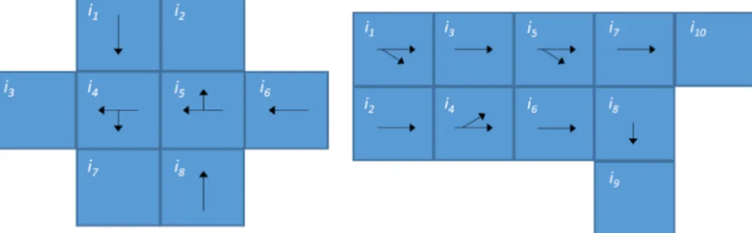
4. Adaptation of the elaborated model, numerical case studies To illustrate the applicability of the elaborated model, two numerical case studies have been conducted using the MATLAB software. The first example has been solved on a transport network segment representing the intersection of a one-lane and a two-lane road section. In the second example, the applicability of lane changes has been demonstrated. The results of the network identification and partition process are illustrated inFig. 1.

In our numerical examples, only passenger vehicles have been considered, and therefore 5 m long locations have been used for

140

(6)

Fig. 1. Locations of road network in the case studies (first case study on left side, second is on right side).

Table 1

Initial data of case studies.

First case study Second case study

m 6 5

t 6 6

o 8 10

v_limit 15 m/s 15 m/s

acc_limit 10 m/s² 10 m/s²

dec_limit 10 m/s² 10 m/s²

Origin Destination Origin Destination

k=1 1 7 1 9

k=2 1 3 1 10

k=3 8 2 2 10

k=4 8 3 2 10

k=5 6 3 2 9

k=6 6 7 – –

Table 2

Results of optimization.

First case study Second case study

Route Route

k=1 i1-i1-i7-i7-i7-i7 i1-i1-i5-i9-i9-i9

k=2 i1-i3-i3-i3-i3-i3 i1-i5-i10-i10-i10-i10

k=3 i8-i2-i2-i2-i2-i2 i2-i2-i4-i5-i10-i10

k=4 i8-i8-i5-i3-i3-i3 i2-i2-i2-i4-i5-i10

k=5 i6-i6-i6-i6-i5-i3 i2-i6-i9-i9-i9-i9

k=6 i6-i6-i6-i5-i7-i7 –

f_obj 118,33 170

segmentation. The initial data and results have been summarized inTables 1and2.

It is possible to solve the predefined optimization problem effectively by using the developed model. Computational time was 1,51 s in the first case and 5,48 s in the second case. The applied computer can be characterized with the following parameters: Intel(R) Core(TM) i7-2620M CPU (2,70 GHz) and 4 GB RAM.

None of the vehicles act in contravention of the defined safety constraints (i.e., velocity, acceleration, and deceleration limits).

Only one vehicle is located at any position at the same time instant, except the origin and destination locations. Furthermore, none of the vehicles cross the route of another vehicle at the same time step. The process ensured that the emerged transport demands had been satisfied efficiently and safely.

5. Model reduction orientations — possibilities to improve the efficiency of the model

The number of variables and constraints significantly influ- ences the developed method’s efficiency and applicability. To investigate this, the detailed summary of these numbers has been elaborated inTable 3, considering the previously introduced parameters (k=1. . .m;j=1. . .t;i=1. . .o).

Based on the structure of the introduced equalities and inequalities, we can conclude that the number of locations has an outstandingly significant impact on the computational complexity of the given problem.

To reduce the number of variables, it seems to an obvious solution to merge the neighboring locations. However, in this case, the locations may have larger extent, which would result in a less efficient traffic-control process. Since, in this case the vehicles would occupy a larger area in a given time step, which could not be used by any other vehicle in the given time step, even if there would be enough space to cross for two or more vehicles as well.

Similarly, if we extend the length of a unit time step, it can reduce the number of variables. However, the efficiency of the control process would be influenced disadvantageously as well.

Instead of the previously introduced orientations, the reduction of the number of constraints can lead to better tractability without threatening the efficiency of the control process.

Considering the data of the introduced case studies (see Table 1), the total numbers of equalities and inequalities are 334.213 in the case of the first case study and 543.141 in the second case study.

Accordingly, due to the numerous redundant boundary conditions, the number of equalities and inequalities can be decreased without threatening the feasibility of the solution related to the given problem.

We provide one example of the reduction regarding the inequalities related to the allowed maximum speed of the vehicles (Eqs. (9), (11), (12), (14), (16)). In the case of the mentioned boundary conditions, only those cases should be investigated, where shortest routes between the compared locations can be traveled in the successive time steps taking into account the allowed maximum speed.

As it can be observed, generally, the consideration of the speed limit can result two types of reduction in the number of constraining inequalities. On the one hand, in the case of the inequalities representing the speed limit (Eq.(9)), the constraints should only be taken into account if the distance between the investigated origin and the destination location is larger than the travelable distance in a unit time step.

On the other hand, in the case of the inequalities representing the acceleration, deceleration limits and prohibition of unsafe crossing (Eqs.(11),(12),(14),(16)), the constraints should only be considered if the travelable distance in a unit time step is larger than or equal to the distance between the investigated origin and the destination location.

For first group (Eq.(9)), it is not necessary to consider those target locations which are not affected by the given limitations.

In this case, the reduced number of the considerable locations is indicated by z₁. For the second group, (Eqs.(11), (12), (14), (16)), it is unnecessary to consider those target locations that are already excluded by the speed limit conditions. These locations are too far away. Due to the considerably limited size of the

(7)

Table 3

Number of variables and equations of the elaborated model.

Equation Number Explanation

Eq.(9) m∗(^t−1)∗o² m∗(^t−1)∗o∗z1

Eq.(11) m∗(^t−2)∗o³ m∗(^t−2)∗o∗z2∗z2

Eq.(12) m∗o² m∗o∗z2

Eq.(14) m∗(^t−2)∗o³ m∗(^t−2)∗o∗z2∗z2

Eq.(16)

(m 2 )

·(^t−1)·o⁴

(m 2 )

·(^t−1)·o·z3·o·z3

network, the excluded target locations’ effect can be different in the case of the different inequality types. Therefore, in the case of Eqs.(11),(12), and(14), the reduced number of the considerable locations is indicated by z₂. In the case of Eq.(16), the reduced number of the considerable locations is indicated byz₃.

After considering the reduction in the number of constraints related to the speed limit factor, the total numbers of equalities and inequalities are 311.765 in the case of the first case study, and 506.918 in the case of the second case study. Accordingly, the reduction is approximately 7% in both cases. Sincez₁,z₂,z₃ values are not depend of the size of the investigated network, the applied simplification reduced the biquadratic problem to a quadratic problem.

Beyond the presented simplification, there are other reduction possibilities, which can further improve the efficiency of the introduced approach. Accordingly, taking into account the reduction effect of the acceleration factor (Eqs. (9), (11), (12), (14),(16)) or excluding the investigation of non-crossing traffic flows (Eq.(16)) can also lead to a significant improvement in the efficiency.

These results support our assumption that taking into account the mentioned development proposals, the introduced approach can provide a relevant contribution to the field of autonomous transportation control.

6. Conclusions

Based on the literature review it has been pointed out that the research of dynamic traffic assignment and control of autonomous transport is commonly treated separately. However, a clear linkage exists between the two processes. Accordingly, a model has been elaborated in our study to bridge this gap. Our model aims to realize the network-level optimization of traffic demand management through the binary integer modeling of cooperative vehicle control processes, assuming a fully autonomous transport system. The developed model investigates the transport processes on the level of the vehicles. A discrete-time domain was formulated, the road network was partitioned into locations, and the optimal vehicle control problem with the necessary constraints was defined. Other advantages of our approach ensure traffic safety, addresses traffic lane management, and capacity management by positioning AVs individually at each model time step.

The main limitation of the applicability of the developed model arises from the detailed partitioning of the road network.

The process of partitioning and defining orientations is a complex engineering task. The large number of locations, model time steps, and separately controlled vehicles increase the computational complexity significantly. The developed procedure defines each vehicle’s possible routes and compares every possible case at each model time step. Many of these cases are irrelevant that could be ignored, reducing the computational complexity. Accordingly, our further development efforts are directed to the reduction of computational complexity by identifying and eliminating the equations describing irrelevant cases.

Due to the speed limit factor, the number of constraints is reduced by approximately 7%. Beyond the presented simplification, there are other reduction possibilities, which can further improve the efficiency of the introduced approach (e.g., acceleration factor, excluding the investigation of non-crossing traffic flows). Accord- ingly, the achieved results can provide a relevant contribution to the field of autonomous transportation control.

Declaration of competing interest

The authors declare that they have no known competing finan- cial interests or personal relationships that could have appeared to influence the work reported in this paper.

Acknowledgments

The research reported in this paper and carried out at the Bu- dapest University of Technology and Economics was supported by the ‘‘TKP2020, Institutional Excellence Program’’ of the National Research Development and Innovation Office in the field of Artifi- cial Intelligence (BME IE-MI-FM TKP2020). The research reported in this paper was supported by Hungarian Academy of Science (HAS) for providing the Janos BOLYAI Scholarship. Moreover, the authors are grateful for the support of New National Excellence Programme Bolyai+ scholarship.

References

[1] N.H. Amer, H. Zamzuri, K. Hudha, Z.A. Kadir, Modelling and control strategies in path tracking control for autonomous ground vehicles: A review of state of the art and challenges, J. Intell. Robot. Syst. 86 (2017) 225–254,http://dx.doi.org/10.1007/s10846-016-0442-0.

[2] R. Azimi, G. Bhatia, R. Rajkumar, P. Mudalige, Ballroom intersection protocol: Synchronous autonomous driving at intersections, in: 2015 IEEE 21st International Conference on Embedded and Real-Time Computing Systems and Applications, Hong Kong, 2015, pp. 167–175, http://dx.doi.

org/10.1109/RTCSA.2015.20.

[3] L.D. Baskar, B. De Schutter, H. Hellendoorn, Model-based predictive traffic control for intelligent vehicles: Dynamic speed limits and dynamic lane allocation, IEEE Intelligent Vehicles Symposium, Eindhoven, 2008, pp.

174-179.http://dx.doi.org/10.1109/IVS.2008.4621307.

[4] M. Ben-Akiva, A. De Palma, I. Kaysi, Dynamic network models and driver information systems, Transp. Res. A 25 (5) (1991) 251–266,http://dx.doi.

org/10.1016/0191-2607(91)90142-D.

[5] P.M. Bösch, F. Ciari, K.W. Axhausen, Transport policy optimization with autonomous vehicles, Transp. Res. Rec.: J. Transp. Res. Board 2672 (8) (2018) 698–707,http://dx.doi.org/10.1177/0361198118791391.

[6] G.R. Campos, P. Falcone, H. Wymeersch, R. Hult, J. Sjöberg, Cooperative receding horizon conflict resolution at traffic intersections, in: Proceedings of the IEEE Conference on Decision and Control, Los Angeles, CA, 2014, pp.

2932-2937,http://dx.doi.org/10.1109/CDC.2014.7039840.

[7] A. Colombo, D. Del Vecchio, Least restrictive supervisors for intersection collision avoidance: A scheduling approach, IEEE Trans. Autom. Control 60 (6) (2015) 1515–1527,http://dx.doi.org/10.1109/TAC.2014.2381453.

[8] C.F. Daganzo, The cell transmission model: A dynamic representation of highway traffic consistent with the hydrodynamic theory, Transp. Res. B 28 (4) (1994) 269–287,http://dx.doi.org/10.1016/0191-2615(94)90002-7.

[9] C.F. Daganzo, The cell transmission model, part II: Network traffic, Transp.

Res. B 29 (2) (1995) 79–93, http://dx.doi.org/10.1016/0191-2615(94) 00022-R.

[10] K. Dresner, P. Stone, Multiagent Traffic Management: A Reservation-Based Intersection Control Mechanism, in: Proceedings of the The Third Interna- tional Joint Conference on Autonomous Agents and Multiagent Systems, New York, NY, USA, 2004, pp. 530-537. Print ISBN: 1-58113-864-4.

[11] T.L. Friesz, T. Kim, C. Kwon, M.A. Rigdon, Approximate network loading and dual-time-scale dynamic user equilibrium, Transp. Res. B 45 (1) (2011) 176–207,http://dx.doi.org/10.1016/j.trb.2010.05.003.

[12] E.J. Gonzales, C.F. Daganzo, Morning commute with competing modes and distributed demand: User equilibrium, system optimum, and pricing, Transp. Res. B 46 (10) (2012) 1519–1534, http://dx.doi.org/10.1016/j.trb.

2012.07.009.

142

(8)

[13] R. Hult, G.R. Campos, P. Falcone, H. Wymeersch, An approximate solution to the optimal coordination problem for autonomous vehicles at intersections, American Control Conference (ACC), Chicago, IL, 2015, pp. 763-768.

http://dx.doi.org/10.1109/ACC.2015.7170826.

[14] R. Hult, G.R. Campos, E. Steinmetz, L. Hammarstrand, P. Falcone, H.

Wymeersch, Coordination of cooperative autonomous vehicles - toward safer and more efficient road transportation, IEEE Signal Process. Mag. 33 (6) (2016) 74–84,http://dx.doi.org/10.1109/msp.2016.2602005.

[15] G.L. Jia, R.G. Ma, Z.H. Hu, Review of urban transportation network design problems based on citespace, Math. Probl. Eng. (2019)http://dx.doi.org/10.

1155/2019/5735702.

[16] P. Kopelias, D. Elissavet, K. Vogiatzis, A. Skabardonis, V. Zafiropoulou, Connected & autonomous vehicles – environmental impacts – a review, Sci. Total Environ. 712 (2019) 135237,http://dx.doi.org/10.1016/j.scitotenv.

2019.135237.

[17] H. Kowshik, D. Caveney, P.R. Kumar, Provable systemwide safety in intelligent intersections, IEEE Trans. Veh. Technol. 60 (3) (2011) 804–818, Available from:http://dx.doi.org/10.1109/TVT.2011.2107584.

[18] A.Y.S. Lam, Y.-W. Leung, X. Chu, Autonomous-vehicle public transportation system: Scheduling and admission control, IEEE Trans. Intell. Transp. Syst.

17 (5) (2016) 1210–1226,http://dx.doi.org/10.1109/TITS.2015.2513071.

[19] H.K. Lo, W.Y. Szeto, A cell-based variational inequality formulation of the dynamic user optimal assignment problem, Transp. Res. B 36 (5) (2002) 421–443,http://dx.doi.org/10.1016/S0191-2615(01)00011-X.

[20] A. Mourad, A. Abbas-Turki, F. Perronnet, J. Wu, A. El Moudni, J. Buisson, R. Zeo, Modeling and controlling an isolated urban intersection based on cooperative vehicles, Transp. Res. C 28 (2013) 44–62,http://dx.doi.org/10.

1016/j.trc.2012.11.004.

[21] G. Pauer, Á. Török, Comparing system optimum-based and user decision- based traffic models in an autonomous transport system, Promet - Traffic Transp. 31 (5) (2019) 581–591,http://dx.doi.org/10.7307/ptt.v31i5.3151.

[22] S. Peeta, A. Ziliaskopoulos, Foundations of dynamic traffic assignment: the past, the present and the future, Netw. Spat. Econ. 1 (2001) 233–265, http://dx.doi.org/10.1023/A:1012827724856.

[23] L. Schewe, M. Schmidt, D. Weninger, A decomposition heuristic for mixed- integer supply chain problems, Oper. Res. Lett. 48 (3) (2020) 225–232, http://dx.doi.org/10.1016/j.orl.2020.02.006.

[24] Y. Shen, H. Zhang, J. Zhao, Integrating shared autonomous vehicle in public transportation system: A supply-side simulation of the first-mile service in Singapore, Transp. Res. A 113 (2018) 125–136,http://dx.doi.org/10.1016/j.

tra.2018.04.004.

[25] M.G. Speranza, Trends in transportation and logistics, European J. Oper.

Res. 264 (3) (2018) 830–836,http://dx.doi.org/10.1016/j.ejor.2016.08.032.

[26] A. Sterling, P. Steven, T. Pilutti, K. Iagnemma, An optimal-control- based framework for trajectory planning, threat assessment, and semi- autonomous control of passenger vehicles in hazard avoidance scenarios, Int. J. Veh. Auton. Syst. 8 (2) (2010) 190–216,http://dx.doi.org/10.1504/

IJVAS.2010.035796.

[27] W.Y. Szeto, H.K. Lo, A cell-based simultaneous route and departure time choice model with elastic demand, Transp. Res. B 38 (7) (2004) 593–612, http://dx.doi.org/10.1016/j.trb.2003.05.001.

[28] C.M.J. Tampere, R. Corthout, D. Cattrysse, L.H. Immers, A generic class of first order node models for dynamic macroscopic simulation of traffic flows, Transp. Res. B 45 (1) (2011) 289–309, http://dx.doi.org/10.1016/j.

trb.2010.06.004.

[29] E. Taniguchi, H. Shimamoto, Intelligent transportation system based dynamic vehicle routing and scheduling with variable travel times, Transp.

Res. C 12 (3–4) (2004) 235–250, http://dx.doi.org/10.1016/j.trc.2004.07.

007.

[30] T. Tettamanti, I. Varga, Z. Szalay, Impacts of autonomous cars from a traffic engineering perspective, Period. Polytech. Transp. Eng. 44 (4) (2016) 244–250,http://dx.doi.org/10.3311/PPtr.9464.

[31] O. Törő, T. Bécsi, S. Aradi, Design of lane keeping algorithm of autonomous vehicle, Period. Polytech. Transp. Eng. 44 (1) (2016) 60–68,http://dx.doi.

org/10.3311/PPtr.8177.

[32] J. Wahle, A.L.C. Bazzan, F. Klügl, M. Schreckenberg, Decision dynamics in a traffic scenario, Physica A 287 (3–4) (2000) 669–681,http://dx.doi.org/

10.1016/S0378-4371(00)00510-0.

[33] S.T. Waller, A.K. Ziliaskopoulos, A combinatorial user optimal dynamic traffic assignment algorithm, Ann. Oper. Res. 144 (2006) 249–261, http:

//dx.doi.org/10.1007/s10479-006-0013-z.

[34] I. Yperman, The Link Transmission Model for dynamic network loading, Open Access Publ. from Kathol. Univ. Leuven, 2007.

[35] X. Zhang, S.T. Waller, Implications of link-based equity objectives on transportation network design problem, Transportation 46 (2018) 1559–1589, http://dx.doi.org/10.1007/s11116-018-9888-1.

[36] F. Zhu, S.V. Ukkusuri, Accounting for dynamic speed limit control in a stochastic traffic environment: A reinforcement learning approach, Transp.

Res. C 41 (2014) 30–47,http://dx.doi.org/10.1016/j.trc.2014.01.014.

[37] F. Zhu, S.V. Ukkusuri, A linear programming formulation for autonomous intersection control within a dynamic traffic assignment and connected vehicle environment, Transp. Res. C 55 (2015) 363–378,http://dx.doi.org/

10.1016/j.trc.2015.01.006.

[38] M. Zöldy, Investigation of autonomous vehicles fit into traditional type approval process, Proceedings of ICTTE, Belgrade, Serbia, 2018, pp.

428-432.