A Connected Dominating Set Based on Connectivity and Energy in Mobile Ad Hoc Networks

A Connected Dominating Set Based on Connectivity and Energy in Mobile Ad Hoc Networks

Ali Kies, Zoulikha Mekkakia Maaza, Redouane Belbachir

Department of Data Processing

University of Sciences and the Technology of Oran BP 1505 El M’Naouar, Oran, Algeria

kies_ali@yahoo.fr, mekkakia@univ-usto.dz, belbachir_red@yahoo.fr

Abstract. A connected dominating set (CDS) has been proposed as a virtual backbone for routing in wireless ad hoc networks. Ad hoc networks offer new routing paradigms.

Therefore, the routing operation needs a broadcast algorithm. Broadcasting in an ad hoc network is still an open issue. The main focus here will be on optimizing the energy and the bandwidth utilization for packet diffusion.

In this paper, we describe the Connected Dominating Set-Energy Protocol (CDSEP) for mobile ad hoc networks to optimize broadcast in the network. The key concept used in this protocol is a new distributed algorithm which computes the connected dominating set (CDS) based on node energy and node connectivity. In the CDSEP protocol, the CDS nodes are selected to forward broadcast packets during the flooding process, and the information flooded in the network through these CDS is also about the CDS. Thus, a second optimization is achieved by minimizing the contents of the control packets flooded in the network. Hence, only a small subset of links with the nodes is declared instead of all the links and the nodes. Our simulation experiment results demonstrate that the CDSEP responds well to scaling in terms of broadcast control packet and energy consumption.

Keywords: ad hoc; self-organization; CDS; energy; routing

1 Introduction

An Ad hoc mobile network is a set of mobile nodes which are dynamically and arbitrarily scattered in a manner where the interconnection between the nodes can change constantly. An ad hoc mobile network can be modeled by a graph G = (V, E) [1]. V represents all nodes and E models the connections set that exists between these nodes. If e = (u, v) Є E, this means nodes u and v are able to communicate directly at that moment.

In most cases, the node destination is not in the transmission range of the node source, which implies that data exchange between two nodes (source, destination) may be carried out by intermediate nodes. The management of this routing of data implies the establishment of certain architecture, and one must take account of the mobility of the nodes and fickleness of the physical medium. An ad hoc mobile network must be self-organized to convey the traffic from one point to another.

The self-organization of an ad hoc network allows the creation of a different view of topology radio called virtual topology. This introduces one or more hierarchy levels and facilitates the establishment of the services necessary to the expected network operation, such as the routing [2].

Several techniques have been proposed to optimize flooding with neighborhood knowledge. Link state routing protocols usually provide this information. It is usually obtained by regularly emitting so-called Hello packets containing lists of neighbors.

From a graph theory point of view, the set of nodes that will retransmit a given broadcast packet must form a connected dominating set (CDS).

If V^- is the node set of the CDS, the formal definition is:

   

, / , , ,

/ ,

u V v V

v N u u v V

e route

w e w V

           

In equation (1), V represents all nodes and V^- represents CDS nodes. N(u) is the neighbor set of u.

A connected dominating set is a set of nodes such that any node in the network is a neighbor of some element of the set. It is connected if the sub-graph formed by this set is connected. The connected dominating set property insures that all nodes will receive the packet.

The CDS forwarding rule is that a node retransmits if it has not already received the packet and it is in the connected dominating set.

Moreover, the selection of the connected dominating set must be distributed.

Based on neighborhood knowledge, a node must decide whether or not it is in the dominating set. A CDS is a good candidate of a virtual backbone for wireless networks, because any non-CDS node in the network has 1-hop distance from a CDS node. With the help of the CDS, routing is easier and can adapt quickly to network topology changes.

Routing protocols are used with the aim of discovering the route which exists between the nodes. The principal goal of such a routing protocol is the establishment of the routes which are correct and effective between any pair of nodes, which ensures the exchange of messages in a continuous way.

Ad hoc routing protocols can be classified into three categories: proactive protocols, reactive protocols and hybrid protocols [1].

Proactive (table-driven) routing protocols maintain up-to-date routes between all nodes in the network. This requires each node to maintain some kind of routing table to store routing information. The ability of the protocol to provide routes to mobile nodes depends on the consistency of the routing tables. Therefore, a node noticing a change in network topology must propagate the updated routing information to all other nodes.

In the reactive routing protocol case, when a node wants to communicate with another node, it initiates a specific route discovery process to obtain a valid route.

Hybrid protocols use both proactive and reactive routing protocols. Other types which are based on geographical position are detailed in [3].

2 Related Works

Three types of virtual topologies are defined: CDS (Connected Dominating Set) allows for the collection of the data traffic and forms a network backbone [2].

Cauterization allows for the partition of the network into zones. The third type integrates CDS and clusters.

The first type is based on the construction of a connected dominating set (CDS) as a virtual backbone to convey information in a mobile network.

[4] proposes a localized algorithm for constructing a CDS. The first step of this algorithm is to mark the nodes having at least two neighbors not directly connected as dominant nodes (become node in the CDS). Applying two dominating reducing rules can reduce some redundant nodes in the CDS. In Rule 1, a marked node can unmark itself if another marked node covers it. In Rule 2, a marked node can unmark it, if covered by two other directly connected marked neighbors. Node A is covered by node B, which means all A’s neighbors are a subset of B’s neighbors. Each node learns its neighbor information and status (mark or unmark) before the next reducing process, through broadcasting Hello messages. So it imposes a significant communication overhead, and energy consumption is high. To reduce communication overhead, the algorithm [5]

presents new rules or extended rules to select/reduce the connected set of dominant nodes. In order to prolong the lifespan of each node, the extended rules are based on two approaches, the approach Node-Degree-Based Rules and Energy- level-Based Rules. Also [6] proposes an improved algorithm [4], in which nodes are assumed to have a record key (degree, x, y), and where x and y are location coordinates. This record is used to apply rules 1 and 2, in which they define that a node can unmark itself if it is covered by one or two connected neighbors, no matter whether they are marked or not. [6] proposes the creation of a source oriented CDS in order to optimize the diffusion of information. The authors of [7]

and [8] propose an iterative exploration starting from a leader in the network to

(Dominating Set) construction and its interconnection. A node has one of four following states: initial state, dominating (CDS member), dominated (neighbor of a dominant) and active (in election). An active node that has the highest weight among its active neighbors becomes dominant, and its neighbors become dominated. The weight for the election can take the degree value, node identifier and energy level. There exist other algorithms based on the same approach without the use of a leader, as described in [9]. In [10] they use the concept of multi point relays. The idea of multipoint relays (MPR) is to use the knowledge of two-hop to optimize local broadcast. Thus, each nodes elects a multipoint relays set among its neighbors, allowing it to attain all nodes at two hops. The more formal definition is:

    ^{, 2}     ^{( ( )}   ⁾

m M

u M u N u N u N M with N M N m

   

ò (2)

Where u is a node, M(u) is a multipoint relay set of u, N(u) is a neighbor set of u and N2 (u) is a two-hop neighbors set of u. Only the multipoint relay of u retransmits a message from u.

Among the routing protocols based on virtual topology, we note Optimized Link State Routing (OLSR) based on the concept of multipoint relay (MPR) [11] and Ad hoc On-demand Distance Vector (AODV) based on CDS [1].

The second type is based on the cluster concept. A cluster is a set of remote limited nodes.

In [12], the node that has the smallest identifier among all its neighbors is elected as the cluster-head. The cluster is formed by the cluster-head and all its neighbors.

In [13] this is reversed; the node whose identifier is the highest among all its neighbors becomes the cluster-head. In [14], the election of cluster-heads is based on the degree of connectivity (the neighbor’s number of nodes) instead of the identities of the nodes. In [15], the weight is defined as the speed of each node.

[16] presents a clustering algorithm. This algorithm involves three steps. Group formation involves two tests: test1 on signal strength, and test2 on mobility, with each one a cluster-head for the management of the cluster and overall cluster-head for network management. The cluster-head is the node with the minimal average distance between it and the other nodes of the group. Overall cluster-head is the node that has the maximum of the cluster-head in its field of coverage. This election is made by using the GPS. There exist routing protocols based on this type; we cite the Cluster Based Routing Protocol (CBRP) [17], the zone routing protocol (ZRP) [18] and the Clusterpow protocol [19]. The Clusterpow protocol uses the power of transmission to build the clustering.

Among the algorithms of the third type, [20] presents a distributed algorithm for constructing a CDS in the form of a K-CDS: the distance between a node and the CDS. The construction and interconnection stages are inspired from [7] and [8].The presence of a leader is obligatory in a hybrid network; the access point (AP) may play the role of natural leader [2].If instead there exists no Access Point,

it is necessary to elect a node using the algorithm described in [21]. The clusters election is done only by nodes which are members of CDS. A dominant node that has the highest weight among all its neighbors at K-cluster and K-CDS, where K is a distance, without cluster-head amounts to the cluster-head. The author of [22]

proposes Virtual Structure Routing (VSR) based on the previous virtual topology [20]. In [23], the principle of the algorithm is summarized as follows: Initially, each node in the network selects its preferred node as the diffusion node, the node that ensures a better diffusion in two hops. Then, the diffusion node having an average of choice higher than that of its neighbors is declared as the cluster-head.

The average of choice is the ratio of dominant nodes which are neighbors to a node and choose the same node as diffusion node divided by number of node’s neighbors. Ordinary nodes are always attached to their node of diffusion. These nodes have a null average of choice. A forest is then built by connecting the cluster-heads, the secondary cluster-heads (members of the CDS, but which are not cluster-heads) and ordinary nodes. Afterwards, the algorithm constructs the routing table within the cluster to provide an appropriate structure for each tree.

The latter is located only at the cluster-heads.

3 CDSEP Algorithm

The desired functions of our virtual topology are:

 Leveraging heterogeneity involving more actively the strong nodes in terms of energy,

 Optimizing the flooding in order to prevent the formation of a broadcast storm,

 Creating a logical cutting near to a physical division allowing locating and addressing the nodes.

Naturally, this structure must follow the following properties: strength, persistence, distributive, scalability and low traffic control.

Initially Neighbor discovery CDS construction Figure 1

The construction of virtual topology

Fig. 1 presents an overview of our virtual topology. Nodes initiate a neighbor discovery to discover their neighboring radios. From this neighborhood radio, the CDS is built by electing the dominants and interconnecting them to form a CDS.

For this, we proposed a new distributed algorithm for construction but also maintenance events. The CDSEP algorithm goes through via two stages:

 Creating Dominant nodes (DNs), i.e. CDS nodes via the Hello messages,

 Interconnecting the dominant nodes (DNs) via the IM (Interconnection Message).

3.1 Virtual Topology Based on Connectivity and Energy

The idea of the CDSEP algorithm is to minimize flooding of broadcast messages in the network by reducing duplicate retransmissions. Each node in the network selects a node in its neighborhood which may retransmit its packets. This node is called a dominant node (DN), i.e. a node in the CDS. The DN set creates the virtual topology named the CDSE in the network. Node neighbors which are not CDSE nodes receive and process broadcast messages but do not retransmit broadcast messages received from the node. Each node selects its DN among its one hop neighbors. This DN has the maximum of Selection Parameter (SP).

3.1.1 Selection Parameter

The selection parameter (SP) is a parameter which enters decision making to build our virtual topology based on CDS and Energy named CDSE (CDS-Energy). For this, we must study all possible values of this parameter. The selection parameter is calculated from two parameters, a parameter related to the node energy and the other related to the network called the connectivity, i.e. the degree of node in the network, by the following equation (3):

    ^*    

0 1 0 0

i i

i

E t log C t SP t 

(3) SP_i(t):Selection parameter of node i at time t,

E_i(t):Energy of node i at time t in Joule, C_i(t):Degree of node i at time t.

Table 1 shows the different states of selection parameter, and shows six cases of the Selection Parameter. In case 1, node i has a value of SP null because node i has a value of energy null. In case 2, node i has value of Connectivity null, so this node is located in the border of the network. Therefore, this node does not participate in the construction of the CDS (not a candidate to be a CDS node).

Table 1 Different states of SP

E(j) C SP

1

if E

 0

 C

SP

 0

2

 E

If C

 1 SP

 0

3

if E

 E

and C

 C

SP

 SP

4

if E

> E

and C

 C

SP

 SP

5

if E

 E

and C

 C

SP

 SP

6

if E

 E

and C

 C

SP

 SP

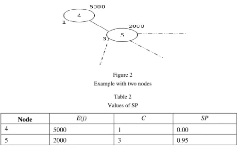
Fig. 2 shows this case: node 1 has a value of SP₁ (SP of node 1) equals zero because this node has a connectivity value C₁=1 (connectivity of node 1 equals 1), i.e. has a neighbor; and the other node 2 has C₂=3 and E₂=2000 (energy of node 2 equals 2000), and when we apply the equation (3) it gives SP₂ =0, 95 as the Table 2 shows.

For the third case, when the energy and connectivity of node i and node j are equal, the SP of node i and node j are also equal.

Figure 2 Example with two nodes

Table 2 Values of SP

Node E(j) C SP

4 5000 1 0.00

5 2000 3 0.95

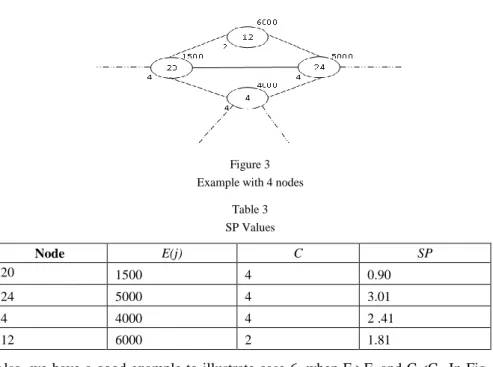
To illustrate case 4 and case 5, we use Fig. 3 and Table3. We note that SP₂₄ equals 3.01, superior to SP₄ equal 2.41 because E₂₄>E₄ and C₂₄ = C₄.

Figure 3 Example with 4 nodes

Table 3 SP Values

Node E(j) C SP

20 1500 4 0.90

24 5000 4 3.01

4 4000 4 2 .41

12 6000 2 1.81

Also, we have a good example to illustrate case 6, when E_i>E_j and C_i<C_j. In Fig.

3, node 12 has E₁₂= 6000 and C₁₂= 2, and node 4 has C₁₂=4 and E₁₂ =4000, which implies SP₄=2, 41 > SP₁₂=1, 81, as Table 3 shows.

The formula can provide a significant value, taking into account the difference between the two parameters energy and connectivity. So, this formula gives a fair value without neglecting any parameter.

The Dominant Node (DN) of node n is denoted DN (n). Each node maintains information about DN.

The DN is recomputed when a change in the SP of a neighborhood is detected or a new neighbor with a SP max is added; a node obtains this information from the periodic Hello messages received from the neighbors.

3.1.2 Process Hello Messages

Each node broadcasts Hello messages containing information about its neighbors and their link status. The link status can be "CDSE" or "S". S is a link of type Symmetric and indicates that the link has been verified to be bidirectional.

"CDSE" indicates that a node is selected by the sender as a DN and it is a link of type Symmetric.

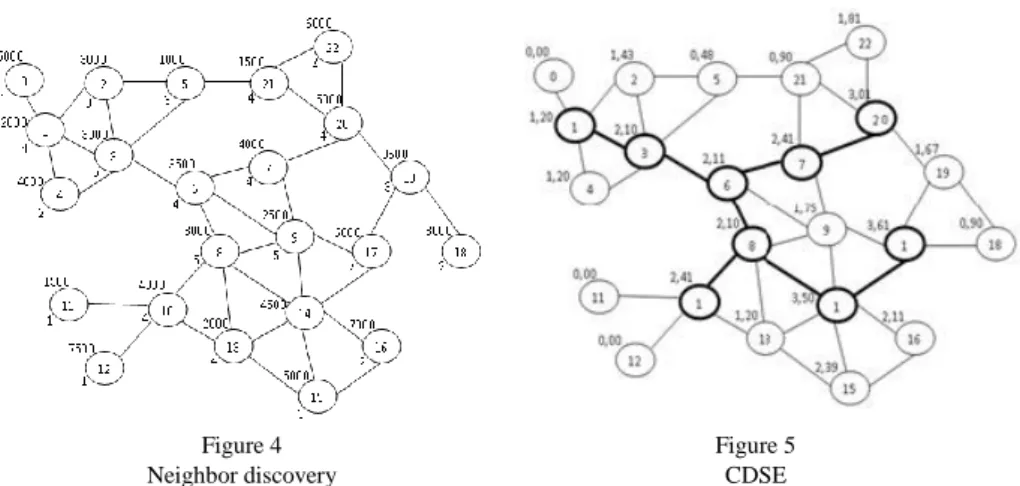
Figure 4 Neighbor discovery

Figure 5 CDSE

In Fig. 4, nodes initiate a neighbor discovery to discover their neighbor. From this neighborhood, the virtual topology is built in a distributed manner. Electing dominants and interconnecting them to form a connected virtual topology, i.e.

connected dominating set-Energy (CDSE), as Fig. 5 shows.

A Hello message contains:

 SP value of sender node,

 A neighbor list, with type of link.

After receiving a Hello message, each node maintains a Neighbor table in which it records the information about its neighbors, its SP, the status of the link with this neighbor, a list of two hop neighbors that this one hop neighbor gives access to, and an associated holding time. The holding time is the lifetime of the neighbor table entry. The information is recorded in the Neighbor table as a neighbor entry, with the field names as shown in Table4:

Table 4 The neighbor table entry

Address of neighbor SP of neighbor Link status 2 hop list Holding time

Based on the information obtained from the Hello messages, each node constructs its CDSE table. In the CDSE table, a node registers the addresses of those one-hop neighbor nodes, and the latter selects the node as a DN.

The CDSE table entry may have the following format in Table 5:

Table 5 The CDSE table entry Node address Holding Time

3.2 Interconnecting Dominant Nodes (DNs)

In order to interconnect the CDSE nodes, each dominant node (DN) broadcasts specific messages called Interconnection Messages (IM). IM messages are forwarded to all nodes of the network, an advantage specific to CDSE nodes. The CDSEP protocol enables a better scalability in the distribution of topology information.

An IM message is sent by a node in the network to declare its CDSE table, i.e. the addresses of those one hop neighbor nodes which have selected the node as a DN.

The information diffused in the network by these IM messages will help each node to compute its topology table. The topology table gives a global overview of the virtual topology CDSE. A node which nobody has selected as a DN cannot generate any IM messages. To reduce the problems of broadcast, each node transmits and retransmits the IM message only if it belongs to the CDSE nodes.

The node belongs to the CDSE nodes if in the neighbor table of this node exists the link of type “CDSE”. When a change to the CDSE table is detected, an IM message should be transmitted.

Each node in the network maintains a Topology table in which it records the information about the virtual topology of the network as obtained from the IM messages. A node records information about the DNs of other nodes in the network in its topology table as a topology table entry, which may have the following format, as Table6 shows:

Table 6 The topology table entry

Node address Dominant Node address Holding time

4 Results

The main purpose of these simulations in NS2 (Network Simulator) is to analyze the behavior of our CDSEP algorithm in various scenarios.

We present simulations that illustrate the results of the CDSEP. We evaluated the CDSEP algorithm with the mobility and density parameter.

Table 7 Simulation parameters

Parameter Value

Number of nodes 20 – 200

Time of simulation 200 s

radio propagation 250 m

Mobility 10 m/s

Degree Between [1,10]

Interval Hello message 2 s

Interval IM message 5 s

The first aspect we notice is the CDSE size (the number of dominants nodes according to the network size). In Fig. 6, we notice a decrease in the number of dominant nodes in CDSE. This number increased from 7 to 43, in the case when we increase the network topology size from 20 to 200 nodes, but not exceeding 22% of dominant nodes overall network nodes. On the other hand, in OLSR this rate reaches 77% MPR number, by applying the equation (6) as Fig. 7 shows.

Such that:

dominant nodes Dominant rate

network size



Figure 6

Average number of dominant nodes in CDSE (CDSEP) and in MPR (OLSR)

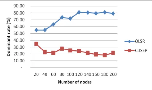
The same comments apply to Fig. 8, which shows the stability of dominant rate about 22% for CDSEP and 77% for OLSR, in all scenarios from 20to200 nodes.

Consequently, the CDSEP protocol adapts well with high density networks. A reduced number of dominant nodes optimize the diffusion in the network.

Figure 7 Rate of dominant nodes

Figure 8

Dominant rates of CDSE and MPR

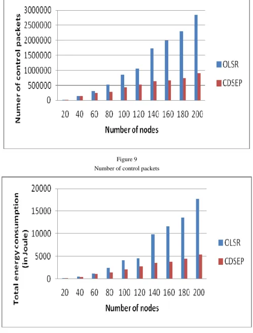
We notice in Fig. 9, the CDSEP reduced the number of control packets generated in the network over OLSR.

When the number of nodes increases, the number of OLSR control packets increases. Consequently, the control traffic decreases in CDSEP, inducing a reduction of energy consumption in the network as Fig. 10 shows.

Figure 9 Number of control packets

Figure 10 Energy consumption

Finally, Fig. 11 shows the rate in terms of control packets and the energy consumed between OLSR and CDSEP, the rate of control packet is calculated using the equation (7):

number of OLSR control parquets

Control packet rate (7)

Figure 11

Control packet and energy consumed report And for consumption energy by applying equation (8):

energy consumed in OLSR Energy consumption rate

energy consumed in CDSE

 (8)

We note that the CDSEP is 3times better for a topology of 180 nodes than the OLSR in terms of the diffusion control packet and energy consumption. As an example, in the OLSR, each node in a topology of 180 nodes consumes an average of 0.38 joules per second, compared to the CDSEP, which consumes 0.12 joules per second.

Conclusion

In this paper, we proposed a distributed algorithm for computing a connected dominating set based on the degree and energy of the node. This information can be contained in hello packets that nodes periodically broadcast to their neighbors.

The CDSE nodes should be responsible for broadcasting packets of other nodes in addition to its own packets, and their energy consumption is high. So it is desirable in selecting nodes for CDSE that we consider the residual energy in the node.

Our contribution, the CDSEP, allows for building a virtual topology based on connectivity and energy. This topology reacts well to scaling, i.e. the rate of control packet to build and interconnect and it is scalable to optimize energy consumption in the network. This structure also allows the participation of the strongest nodes in terms of energy, which permits a longer life of the virtual topology and also permits the building of a connected dominating set, because the dominant nodes are chosen according to the connectivity parameter.

This study laid the foundation for proposing a new routing protocol, and that is the subject of our next work.

Acknowledgments

This work is part of the CAPRAH project 08/U311/4966, supported by the Algerian Ministry of Higher Education and Scientific Research.

References

[1] S. K. Sarkar, T. G. Basavaraju, C. Puttamadappa: Ad Hoc Mobile Wireless Networks, Principles, Protocoles, and Application. Taylor edition (2008) [2] P. Santi,” Topology Control in Wireless Ad Hoc and Sensor Networks,”

Wiley edition (2005)

[3] M. L. M. Kiah, L. K. Qabajeh and M. M. Qabajeh: Unicast Position-based Routing Protocols for Ad-Hoc Networks. Acta Polytechnica Hungarica, Vol. 7, No. 5, 2010

[4] J. Wu, H. Li: On Calculating Connected Dominating Set for Efficient Routing in Ad Hoc Wireless Networks. In Proc. of the 3^rd Int’l Workshop on Discrete Algorithms and Methods for Mobile Computing and Communication (1999)

[5] H. Li, J.Wu: Dominating-Set-based Routing in Ad Hoc Wireless Networks.

In Proc. of International Workshop on Discrete Algorithms and Methods for Mobile Computing and Communications(DIAL'M) USA, August (1999)

[6] I. Stojmenovic, M. Seddigh, J. Zunic: Dominating Sets and Neighbor Elimination-based Broadcasting Algorithms in Wireless Networks. IEEE Transactions on Parallel and Distributed Systems, January (2002)

[7] B. Liang, Z. J. Haas: Virtual Backbone Generation and Maintenance in Ad Hoc Network Mobility Management. In Proc. of INFOCOM, March (2000) [8] X. Cheng, D. Du: Virtual Backbone-based Routing in Multihop Ad Hoc

Wireless Networks. Technical Report 02-002, University of Minnesota, Minnesota, USA, January (2002)

[9] B. Ryu, J. Erickson, J. Smallcomb, S. Dao: Virtual Wire for Managing Virtual Dynamic Backbone in Wireless Ad Hoc Networks. In Proc. of International Workshop on Discrete Algorithms and Methods for Mobile Computing and Communications (DIAL'M), Seattle, USA, August (1999) [10] T. Clausen, P. Jacquet, A. Laouiti, P. Muhlethaler, A. Qayyum and L.

Viennot: Optimized Link State Routing for Ad hoc Networks, IEEE INMIC, Pakistan (2001)

[11] P. Jaquet, P. Muhlethaler, A. Qayyum: Optimized Link State Routing (olsr) Protocol. Internet Draft, draft-ietf-manet-olsr-01.txt, February (2000)

[12] A. Ephremides, J. Wieselthier, D. Baker: A Design Concept For Reliable Mobile Radio Network With Frenquency Hopping Signaling. Procedings of the IEEE, Vol. 75, No. 1, January (1987)

[13] B. Haggar: Self-Stabilizing Clustering Algorithm for Ad Hoc Networks.

Wireless and Mobile Communications, 2009. ICWMC '09. Fifth International Conference, Cannes, La Bocca (2009)

[14] H. Taniguchi, M. Inoue, T. Masuzawa, H. Fujiwara: Clustering Algorithms in Ad Hoc Networks. Electronics and Communications in Japan (2005) [15] S. Basagni: Distributed Clustering Ad Hoc Networks. In Proceedings of the

IEEE International Symposium on Parallel Architectures, Algorithms, and Networks (I-SPAN) (1999)

[16] N. Benaouda, HervéGuyennet, Ahmed Hammad and M. Mostefai: A New Two Level Hierarchy Structuring for node Partitionning in Ad Hoc Networks. In Proceedings of ACM Symposium on Applied Computing, SAC'10, Zurich, Switzerland, pp. 719-726, March (2010)

[17] M. Jiang, J. Li, Y. C. Tay: Cluster-based Routing Protocol (CBRP). Internet Draft, draft-ietf-manet-cbrp-spec-01.txt, 14 August (1999)

[18] J. Haas, R. Pearlman: The Zone Routing Protocol (ZRP) for Ad Hoc Networks. Internet Draft, draft-haas-zone-routing-protocol-00.txt, November (1997)

[19] P. Santi: Topology Control in Wireless Ad Hoc and Sensor Networks.

Wiley edition (2005)

[20] F. Theoleyre and F. Valois: A Virtual Structure for Mobility Management in Hybrid Networks. In Wireless Communications and Networking Conference (WCNC) IEEE, Vol. 5, pp. 1035-1040, Atlanta, USA, March (2004)

[21] N. Malpani, J. L. Welch, N. Vaidya: Leader Election Algorithms for Mobile Ad Hoc Networks. In International Workshop on Discrete Algorithms and Methods for Mobile Computing and Communications (DIALM), USA, August (2000)

[22] F. Theoleyre and F. Valois: Virtual Structure Routing in Ad Hoc Networks.

In International Conference in Communications (ICC), IEEE, Vol. 2, pp.

3078-3082, Seoul, Korea, May (2005)

[23] K. Drira, H. Khedouci, N. Tabbane:Virtual Dynamic Topology for Routing in Mobile Ad Hoc Networks. Proceedings of the International Conference on Late Advances in Networks (ICLAN'2006) pp. 129-134, Paris France (2006)