BOUNDARY CONDITIONS
PETRA CSOM ´OS, MATTHIAS EHRHARDT, AND B ´ALINT FARKAS
Abstract. In this work we study operator splitting methods for a certain class of coupled abstract Cauchy problems, where the coupling is such that one of the sub-problems prescribes a “boundary type” extra condition for the other one. The theory of one-sided coupled operator matrices provides an excellent framework to study the well-posedness of such problems. We show that with this machinery even operator splitting methods can be treated conveniently and rather efficiently. We consider three specific examples: the Lie (sequential), the Strang, and the weighted splitting, and prove the convergence of these methods along with error bounds under fairly general assumptions.
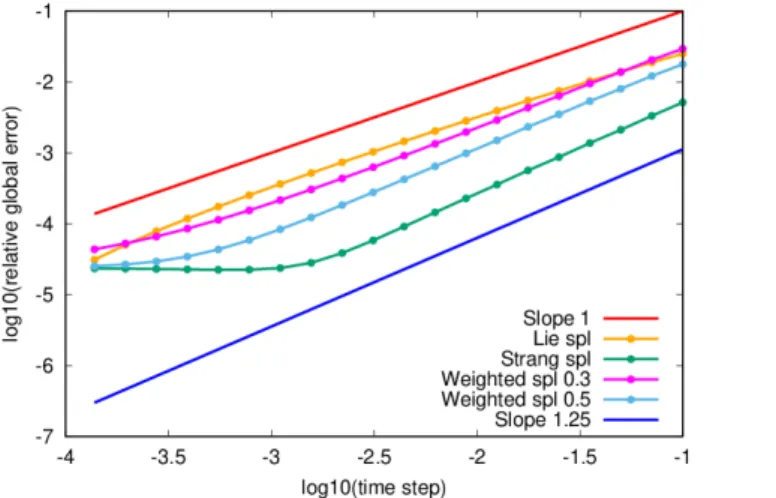
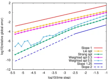
Simple numerical examples show that the obtained theoretical bounds can be computationally realised.
1. Introduction
Operator splitting procedures provide an efficient way of solving time-dependent differential equations which describe the combined effect of several processes. In this case the operator describing the time-evolution is the sum of certain sub-operators corresponding to the different processes. The main idea of operator splitting is that one solves the sub-problems corresponding to the sub-operators separately, and constructs the solution of the original problem from the sub-solutions.
Depending on how the sub-solutions define the solution itself, one can distinguish several operator splitting procedures, such as sequential (proposed by Bagrinovskii and Godunov in [3]), Strang (proposed by Strang and Marchuk in [53] and [48]), or weighted ones (see e.g. in Csom´os et al. [14]). An application of sequential splitting, for instance, results in the subsequent solution of the sub-problems using the previously obtained sub-solution as initial condition for the next sub-problem.
Although operator splitting procedures enable the numerical treatment of complicated differential equations, their application leads to an approximate solution which usually differs from the exact one. The accuracy can be increased by considering the sequence of the sub-problems on short time intervals in a cycle, which will in turn increase the computational effort. However, the analysis of the error, caused by the use of operator splitting, stands in the main focus of related research. For general overviews on splitting methods we refer the interested reader to the vast literature. For instance, Bjørhus analysed the consistency of sequential (Lie) splitting in an abstract framework in [9], Sportisse considered the stiff case in [52], Hansen and Ostermann also treated the abstract case in [28], while B´atkai et al. applied the splitting methods for non-autonomous evolution equations in [7]. Error bounds in the abstract setting were proved by Jahnke and Lubich in [36] for the Strang splitting. While Hansen and Ostermann in [29] have treated higher order splitting methods. A survey can be found in [22] by Geiser.
Another challenging issue is what kinds of processes of the sub-operators describe. They can e.g. correspond to various physical, chemical, biological, financial, etc. phenomena. Hundsdorfer and Verwer analysed the splitting of advection–diffusion–reaction equations in [35, Chapter IV], Dimov et al. solved air pollution transport models in [15], Jacobsen et al. considered the Hamilton–Jacobi equations in [38], Holden et al. partial differential equations with Burgers nonlinearity in [34], while in [12] Csom´os and Nickel and in [5, 6] B´atkai et al. applied splitting methods for delay equations. Splitting methods for Schr¨odinger equations are treated, e.g., in Hochbruck et al.
[37], Caliari et al. [10].
The sub-operators can also correspond to the change (derivative) with respect to various spatial coordinates or other variables, as Hansen and Ostermann has studied in [28], [30]; or for the case of Maxwell equations, see, e.g., Jahnke et al. [33] or Eilinghoff and Schnaubelt [16]. Furthermore, the sub-problems may originate from other (mathematical) properties of the problem itself, as in the present case of dynamical boundary problems.
We emphasise that the analysis and the numerical treatment of dynamical boundary problems has been attracting the attention of several researchers recently, cf. the work of Hipp [31, 32] for wave-type equations or Knopf et al.
[40, 39, 41] on the Cahn–Hilliard equation or Kov´acs et al. [42] and Kov´acs, Lubich [43] on parabolic equations.
The literature is extensive, and we mention some very recent papers by Altmann [1], Epshteyn, Xia [20], Fukao et al. [21], Langa, Pierre [44], and refer to the references therein.
2020Mathematics Subject Classification. 47D06, 47N40, 34G10, 65J08, 65M12, 65M15.
Key words and phrases. operator splitting, Lie and Strang splitting, Trotter product, abstract dynamical boundary problems, error bound.
1
arXiv:2004.13503v2 [math.AP] 20 May 2021
In the present work we focus on theabstract setting of coupled Cauchy problems, where one of the subproblems provides an extra condition, of boundary type, to the other. We consider equations of the form:
(1.1)
˙
u(t) =Amu(t) fort≥0, u(0) =u0∈E,
˙
v(t) =Bv(t) fort≥0, v(0) =v0∈F, Lu(t) =v(t) fort≥0,
where E andF are Banach spaces over the complex fieldC,AandB are (unbounded) linear operators on Eand F, respectively. The coupling of the two problems involves the unbounded linear operator L acting between E andF. Moreover, this coupling is of “boundary type”, i.e., as concrete examples we have in mind problems of the following form:
˙
u(t) = ∆Ωu(t), u(0) =u0∈L2(Ω), (1.2)
˙
v(t) = ∆∂Ωv(t), v(0) =v0∈L2(∂Ω), (1.3)
u(t)|∂Ω=v(t),
where Ω is a bounded domain inRdwith sufficiently regular boundary andAm= ∆Ω,B= ∆∂Ωare the (maximal) distributional Laplace and Laplace–Beltrami operators restricted to the respective L2-space. In this example L denotes the trace operator (the precise ingredients will be discussed in Example 2.7 below.)
It is a natural idea for the numerical treatment of (1.2)–(1.3) to apply operator splitting methods, i.e. to treat the first and second equations separately, see also in [43]. The purpose of this work is to investigate such possibilities, and as a splitting strategy we propose the following steps:
(1) Choose a time stepτ >0.
(2) Solve the second equation (1.3) with the initial conditionv(0) =u0|∂Ω=v0, set v1:=v(τ).
(3) Solve the first equation (1.2) on [0, τ] with the inhomogeneous boundary condition u(t)|∂Ω=v1 and the initial conditionu(0) =eu0. The method determines howeu0 is calculated fromu0 (andv0), and in general ue0 does not need to equalu0. Setu1=u(τ).
(4) The new initial condition for equation (1.3) is thenu1|∂Ω=v1. (5) Iterate this procedure forn∈Ntime steps.
The aim of this paper is to formulate this splitting method as an operator splitting in an abstract operator semigroup theoretic framework and investigate its convergence properties. The method then becomes applicable for a wider class of equations than in (1.1). Our choice for the auxiliary, modified initial valueeu0, in Step 3 above, is motivated by this approach. Indeed, the abstract theory will immediately yield the convergence of the method as an instance of the Lie–Trotter formula. However, we shall briefly touch upon other possible choices for ue0 as well.
As a matter of fact our proposed methods, at a first sight, will be slightly different in that we decompose the system in not two but three sub-problems. This idea is nicely illustrated in the above example of diffusion:
We separate the dynamics in the domain and assume homogeneous boundary conditions, the dynamics on the boundary, and as the third component the interaction between the two dynamics, i.e., how the boundary dynamics is fed into the domain. In fact, this decomposition is responsible for the modified formue0 of the initial condition.
This approach will also have the advantage that the internal and boundary dynamics are completely separated.
Hence well-established methods can be used for solving each of the subproblems. We also note that the splitting approach here gives a way to parallelisation of the solution to the subproblems.
This work is organised as follows. In Section 2 we recall the necessary operator theoretic background for this programme and in Section 3 we introduce the different splitting approaches for the dynamical boundary conditions:
the Lie splitting, the Strang splitting and the weighted splitting. We also prove the convergence of these methods under fairly general assumptions. Section 4 contains error bounds for the above mentioned splitting methods.
Finally, in Section 5 we illustrate the proposed methods by numerical examples, and show that the analytically proved error bounds are realised computationally, too.
2. Abstract dynamical boundary conditions
Before discussing splitting methods in more detail let us briefly recall a possible approach for treating such abstract dynamical boundary value problems. The abstract treatment of boundary perturbations, i.e., techniques for altering the domain of the generator of a C0-semigroup goes back to the work of Greiner [26]. Many results have been building on his theory, and our main sources for describing the abstract setting will be the works by Casarino, Engel, Nagel, and Nickel [11] and Engel [17, 18]. In [11] the following set of conditions were posed for treating the well-posedness of the problem (1.1).
Hypothesis 2.1. TheC-vector spacesEandF are Banach spaces.
(i) The operators Am: dom(Am)⊆E→E andB: dom(B)⊆F →F are linear.
(ii) The linear operatorL: dom(Am)→F is surjective and bounded with respect to the graph norm of Am on dom(Am).
(iii) The restrictionA0 ofAmto ker(L) generates a strongly continuous semigroup T0(t)
t≥0onE.
(iv) The operatorB generates a strongly continuous semigroup S(t)
t≥0onF. (v) The operator (matrix) ALm
: dom(Am)→E×F is closed.
Remark 2.2. Consider the following conditions.
(i’) The operator Am: dom(Am)⊆E→E is linear.
(ii’) The linear operatorL: dom(Am)→F is surjective.
(iii’) L: dom(Am)→F has a bounded right-inverseR:F→E with rg(R)⊆ker(Am).
(iv’) The restriction A0 of Am to dom(A0) := ker(L) is (boundedly) invertible (i.e., 0 ∈ρ(A0); in general, it is sufficient to assume that the resolvent setρ(A0) is non-empty).
Under these assumptions ALm
: dom(Am)→E×F is closed. To see this, we first recall from the proof of Lemma 2.2 in [11] that in this case
dom(Am) = dom(A0)⊕ker(Am).
We also repeat the quick argument for this, taken from [11]: Forx∈dom(Am) we have
x=A−10 Amx+ (x−A−10 Amx) with A−10 Amx∈dom(A0), x−A−10 Amx∈ker(Am).
Furthermore, ifx∈dom(A0)∩ker(Am), thenA0x=Amx= 0, and x= 0 follows by 0∈ρ(A0).
Now, let xn ∈ dom(Am) be with xn → x, Amxn → y in E and Lxn → z in F as n → ∞. We need to show x ∈dom(Am), Amx=y, Lx =z. For each n∈ Nwrite xn =x0n+x1n with x0n ∈dom(A0) and x1n ∈ker(Am).
Then Amxn = Amx0n+Amx1n =Amx0n = A0x0n, thus x0n →A−10 y in E as n → ∞. On the other handLxn = Lx0n+Lx1n =Lx1n→z inF asn→ ∞. It follows that
RLxn=RLx1n→Rz ∈dom(Am).
Moreover, fromL(x1n−RLx1n) = 0 we concludex1n−RLx1n∈dom(A0) andA0(x1n−RLx1n) =Amx1n−AmRLx1n= 0, so thatx1n=RLx1n follows. This impliesx−A−10 y=Rz,x∈dom(Am),Amx=y andLx=LRz=z.
In this paper we make the following technical assumption to simplify the things a bit.
Hypothesis 2.3. The operatorsA0 andB are invertible.
However, let us note that for the splitting procedures this makes no theoretical difference, since (for semigroup generators) one always finds sufficiently large λ > 0 such that A0−λ and B −λ become invertible. Then the numerical schemes can be applied in this rescaled situation.
Next, we recall the following definition from [11, Lemma 2.2], and note that under the previous assumption the following operator is bounded
D0:=L|−1ker(A
m): F→ker(Am)⊆E.
(2.1)
The operator D0 is called the abstract Dirichlet operator; the operator L|ker(Am) is indeed invertible, see the mentioned lemma in [11]. We remark that the existence of this Dirichlet operator D0 =:R, a continuous right- inverse to L as in Remark 2.2, is therefore equivalent to the closedness of ALm
(under the assumption that 0∈ρ(A0)).
Remark 2.4. (a) The operatorD0B: dom(B)→E is bounded if dom(B) is supplied with the graph-normk · kB. (b) We have rg(D0)∩dom(A0) ={0}.
Following [11] we introduce the product spaceE×F and the operatorAacting on it as
(2.2) A:=
Am 0
0 B
with dom(A) := x y
∈dom(Am)×dom(B) :Lx=y . Section 1.1 in [51] relates the well-posedness of (1.1) to the generation property of A, see also [50].
The first thing to be settled is therefore, whether the abstract Cauchy problem
˙
u(t) =Au(t), fort≥0, u(0) =u0= (u0, v0)>,
is well-posed in the sense of C0-semigroups, see [19, Section II.6]. In this case the solution satisfiesu(t) =T(t)u0, where (T(t))t≥0is the semigroup generated byA. The problem of well-posedness is solved in [11]. We briefly recall here the following results from Theorem 2.7 in [11] and from its proof.
Theorem 2.5. Let the operators A,D0 be as defined in (2.2)and (2.1)and assume Hypotheses 2.1and 2.3. For y∈dom(B)define
(2.3) Q(t)y=D0S(t)y−T0(t)D0y− Z t
0
T0(t−s)D0S(s)Byds.
Operator Ais the generator of aC0-semigroup if and only if for eacht≥0 the operator (extends to)
(2.4) Q(t)∈L(F, E) and lim sup
t↓0
kQ(t)k<∞.
In this case the semigroup T(t)
t≥0 generated by Ais given by
(2.5) T(t) =
T0(t) Q(t) 0 S(t)
.
The next condition will be important throughout the paper.
Hypothesis 2.6. The operatorA0 generates a bounded analytic semigroup (see [47, 27] for details about analytic semigroups).
If Hypotheses 2.1, 2.3 and 2.6 are fulfilled and alsoB is a generator of an analytic semigroup, then Theorem 2.5 applies and assures that the semigroup (T(t))t≥0 generated byAis analytic too, see [11, Corollary 2.8].
The motivating example from the introduction is discussed in [11, Section 3] in detail. We recall here the ingredients, to illustrate that our proposed methods will be applicable also for this equation.
Example 2.7 (Laplace and Laplace–Beltrami operators). Let Ω be a bounded domain in Rd with boundary∂Ω of class C2.
• E := L2(Ω), F := L2(∂Ω) are the L2-spaces with respect to the Lebesgue and the surface measure, respectively.
• ∆Ωand ∆∂Ωare the (maximal) distributional Laplace and Laplace–Beltrami operators, respectively.
• Am:= ∆Ωwith domain
dom(Am) :={f :f ∈H1/2(Ω) with ∆Ωf ∈L2(Ω)}.
• Lf =f|∂Ωthe trace off ∈dom(Am) on∂Ω.
• B = ∆∂Ωwith domain
dom(B) ={g:g∈L2(∂Ω) with ∆∂Ωg∈L2(Ω}.
Hypotheses 2.1, 2.3, 2.6 are satisfied for these choices. In particular,Agenerates an analytic semigroup onE×F, see [11, Section 3]. We also have the following:
• The Dirichlet operatorD0: L2(∂Ω)→H1/2(Ω) assigns to a prescribed boundary valueg a functionf with f|∂Ω=g(in the sense of traces) and ∆Ωf = 0.
• A0= ∆Dis the Laplace operator with (homogeneous) Dirichlet boundary condition, generating the Dirich- let heat semigroup (T0(t))t≥0on L2(Ω).
• The semigroup (S(t))t≥0 is the heat semigroup on L2(∂Ω).
Example 2.8 (Bounded Lipschitz domains). In this example we indicate that one can relax the smoothness condition on the boundary of the domain from Example 2.7. Let Ω ⊆Rd be a bounded domain with Lipschitz boundary ∂Ω.
(a) Consider the following operators:
• Am= ∆Ωwith domain
dom(Am) :={f :f ∈H1/2(Ω) with ∆Ωf ∈L2(Ω)}.
• Lf =f|∂Ωthe trace off ∈dom(Am) on∂Ω (see, e.g., [49, pp. 89–106]).
ThenLis surjective and actually has a bounded right-inverse R: L2(∂Ω)→ker(Am),
where dom(Am) is endowed with the normu7→ kukH1/2+k∆uk2, see Theorem 3.6 (i) in [8] for precisely this statement (or [25, Lemma 3.1, Theorem 5.3], [24], [49, Theorem 3.37]). The restrictionA0 ofAm to
ker(L) ={f : H1/2(Ω), ∆Ωf ∈L2(Ω), Lf = 0}
is strictly positive, self-adjoint, in particularA0is invertible and generates a bounded analytic semigroup, [25, Theorem 5.1], [24, Theorem 2.11] (see also [8, Theorem 3.6 (v)]). By invoking Remark 2.2 we obtain that
Am L
: dom(Am)→ L2(Ω)×L2(∂Ω) is closed, and altogether that Am and L satisfy the relevant conditions from Hypothesis 2.1.
(b) One can also consider the Laplace–Beltrami operatorB:= ∆∂Ωon L2(∂Ω), which (with an appropriate domain) is also a strictly positive, self-adjoint operator, see [25, Theorem 2.5] or [23] for details.
Summing up, we see that the abstract framework of [11], hence of this paper, covers also some interesting cases of dynamical boundary value problems on bounded Lipschitz domains.
The decisive tool, based on the theory of coupled operator matrices [17, 18], is to bring the formally diagonal operator Awith anon-diagonal domain into an upper triangular form with the state space transformations
R0=
I −D0
0 I
, R−10 =
I D0
0 I
. Accordingly, we obtain the following representation:
(2.6) A=R−10 A0R0,
where
A0=
A0 −D0B
0 B
with dom(A0) = dom(A0)×dom(B), see [11, Lemma 2.6 and the proof of Corollary 2.8].
3. Operator splitting methods for dynamical boundary conditions problems
Since the form of the semigroup (T(t))t≥0 can be rarely determined in practice, our aim is to determine an approximation to it, and denote at time t =kτ the approximation of u(kτ) by uk(τ) for all k∈N. The natural requirement is that the approximate value should converge to the exact one when refining the temporal resolution (letting τ→0). We recall the following definition from [45] due to Lax and Richtmyer.
Definition 3.1 (Convergence). The approximationuk is called convergent to the solutionuof problem (1.1) on [0, tmax] (for giventmax>0) ifu(t) = lim
n→∞un(nt) holds uniformly for allt∈[0, tmax].
Starting from the representation (2.6), we construct approximations of the form
(3.1) uk(τ) :=R−10 T(τ)kR0 uv0
0
,
where the operator T(τ) :E×dom(B)→E×dom(B),τ≥0 describes the actual numerical method, andu(0) = u0= (u0, v0)>. In order to specify the operatorT(τ), we remark that the operatorA0can be written as the sum
A0=:A1+A2+A3, where
A1=
A0 0
0 0
, A2=
0 −D0B
0 0
, A3= 0 0
0 B
, with
dom(A1) = dom(A0)×F, dom(A2) =E×dom(B), dom(A3) =E×dom(B).
We point out that A1 and A3 commute (in the sense of resolvents). From Hypothesis 2.1 and Remark 2.4 we immediately obtain the following proposition.
Proposition 3.2. The operator semigroups(Ti(t))t≥0,i= 1,2,3 given by T1(t) =
T0(t) 0
0 I
, T2(t) =
I −tD0B
0 I
, T3(t) =
I 0 0 S(t)
are strongly continuous onE×dom(B)with generator
A1|E×dom(B),A2 andA3|E×dom(B), respectively.
Here we consider the parts of the respective operators in the space E×dom(B). The semigroups (T1(t))t≥0 and (T3(t))t≥0 are even strongly continuous onE×F. Their generators areA1 andA3, respectively.
In this work we focus on methods (3.1) with the following choices for the operator T(τ):
T[Lie](τ) :=T1(τ)T2(τ)T3(τ) (3.2)
for theLie (or sequential) splitting;
T[Str](τ) :=T1(τ2)T3(τ2)T2(τ)T3(τ2)T1(τ2) (3.3)
for theStrang (or symmetrical) splitting;
T[wgh](τ) := ΘT1(τ)T2(τ)T3(τ) + (1−Θ)T3(τ)T2(τ)T1(τ) (3.4)
for theweighted splitting, where the parameter Θ∈[0,1] is fixed. We note that the case Θ = 1 corresponds to the Lie splitting, while Θ = 0 gives the Lie splitting in the reverse order. Computing the composition of the operators leads to the common form
(3.5) T(τ) =
T0(τ) V(τ) 0 S(τ)
with the operators
Lie splitting: V[Lie](τ) =−τ T0(τ)D0BS(τ), (3.6)
Strang splitting: V[Str](τ) =−τ T0(τ2)D0BS(τ2), (3.7)
weighted splitting: V[wgh](τ) =−τ(ΘT0(τ)D0BS(τ) + (1−Θ)D0B) (3.8)
for allτ >0. The approximation (3.1) requires the powers of the operatorT(τ) to be computed next.
Proposition 3.3. For the operator family T(τ) :E×dom(B) → E×dom(B), τ > 0, from (3.5) we have the identity
T(τ)k=
T0(kτ) Vk(τ) 0 S(kτ)
with
Vk(τ) =
k−1
X
j=0
T0 (k−1−j)τ
V(τ)S(jτ).
(3.9)
Proof. We show the assertion by induction. For k= 1 we have formula (3.5) with V1(τ) =V(τ). If the assertion is valid for some k≥1, then
T(τ)k+1=
T0(kτ) Vk(τ) 0 S(kτ)
T0(τ) V(τ)
0 S(τ)
=
T0 (k+ 1)τ
Vk+1(τ) 0 S (k+ 1)τ
holds with
Vk+1(τ) =T0(kτ)V(τ) +Vk(τ)S(τ)
=T0(kτ)V(τ) +
k−1
X
j=0
T0 (k−1−j)τ
V(τ)S(jτ)S(τ)
=T0(kτ)V(τ) +
k
X
j=1
T0 (k−j)τ
V(τ)S (j−1)τ S(τ)
=
k
X
j=0
T0 (k−j)τ
V(τ)S(jτ).
This proves the assertion for all k∈Nby induction.
The convergence of the approximation relies on the following result.
Proposition 3.4. Under Hypotheses 2.1, 2.3, (2.4) and with the notation in (3.5), the approximation (3.1) is convergent for y∈dom(B) if the condition
(3.10) lim
n→∞Vn(nt)y=− Z t
0
T0(t−s)D0S(s)By ds holds uniformly for tin compact intervals.
Proof. From Proposition 3.3, the approximation has the form
(3.11)
uk(τ) =
I D0
0 I
T0(kτ) Vk(τ) 0 S(kτ)
I −D0
0 I
u0
=
T0(kτ) Vk(τ)−T0(kτ)D0+D0S(kτ)
0 S(kτ)
u0.
By comparing with formula (2.5) and using the relation (2.3), condition (3.10) implies the assertion.
The convergence of the Riemann sums implies our next result concerning the approximation of the convolution in (3.10).
Lemma 3.5. Let tmax ≥ 0, let f: [0, tmax] → L(F, E) be strongly continuous, and let g: [0, tmax] → F be continuous. For eachn∈Nandt∈[0, tmax]define the following expressions
Cn[1](t) := nt
n−1
X
j=0
f (n−j)nt g(jnt),
Cn[2](t) := nt
n−1
X
j=0
f (n−j−12)nt
g (j+12)nt .
Then for j= 1,2 we have that
n→∞lim Cn[j](t) = Z t
0
f(t−s)g(s) ds holds uniformly for t∈[0, tmax].
We can now state the main result of this section concerning convergent approximations of the solution to problem (1.1).
Proposition 3.6. Under Hypotheses 2.1,2.3, and (2.4) the approximations defined in (3.2),(3.3), and (3.4)are convergent for all u0∈E×dom(B).
Proof. It suffices to prove that condition (3.10) holds for the operatorsV(τ) defined in (3.6), (3.7) and (3.8). By Proposition 3.3, we have the following identity for the Lie splitting:
Vk[Lie](τ)y=−τ
k−1
X
j=0
T0 (k−1−j)τ
T0(τ)D0BS(τ)S(jτ)y
=−τ
k−1
X
j=0
T0 (k−j)τ
D0BS (j+ 1)τ y,
for the Strang splitting:
Vk[Str](τ)y=−τ
k−1
X
j=0
T0 (k−1−j)τ
T0(τ2)D0BS(τ2)S(jτ)y (3.12)
=−τ
k−1
X
j=0
T0 (k−j−12)τ
D0BS (j+12)τ y,
and for the weighted splitting:
Vk[wgh](τ)y=−τ
k−1
X
j=0
T0 (k−1−j)τ
ΘT0(τ)D0BS(τ) + (1−Θ)D0B S(jτ)y
=−Θτ
k−1
X
j=0
T0 (k−j)τ
D0BS (j+ 1)τ y
−(1−Θ)τ
k−1
X
j=0
T0 (k−j−1)τ
D0BS(jτ)y
for ally∈dom(B),τ >0, and Θ∈[0,1]. SinceB and the semigroup operatorsS(t) commute on dom(B), we have Vn[Lie](nt)y=−τ
n−1
X
j=0
T0((n−j)nt)D0S((j+ 1)nt)By,
Vn[Str](nt)y=−τ
n−1
X
j=0
T0((n−j−12)nt)D0S((j+12)nt)By,
Vn[wgh](nt)y=−Θτ
n−1
X
j=0
T0((n−j)nt)D0S((j+ 1)nt)By
−(1−Θ)τ
n−1
X
j=0
T0((n−j−1)nt)D0S(jnt)By.
Now, Lemma 3.5 yields the convergence to the convolution in (3.10) for each of these cases.
Remark 3.7. The stability of splitting methods for triangular operator matrices has been studied in [4]. If we write A0=
A0 0
0 B
+
0 −D0B
0 0
=B+A2, thenB with dom(B) =E×dom(B2) generates the strongly continuous semigroup
S(t) =
T0(t) 0 0 S(t)
onE×dom(B). SinceA2 is bounded on this space, by [4, Prop. 2.4] we obtain that for someM ≥0 andω∈R
S(nt)T2(nt)n
L(E×dom(B))≤Meω for every t≥0.
Thus we immediately obtain the convergence of the corresponding Lie splitting procedure onE×dom(B) by the Lie–Trotter product formula, see [19, Section III.5], or [54]. As a matter of fact, in this way we obtain also the generator property ofA0 onE×dom(B) directly, without recurring to [11].
Remark 3.8. Let us comment on the relation between the previously proposed Lie splitting and the one from the introduction. Given u0 ∈ H1/2(Ω) such that v0 = u0|∂Ω belongs to dom(B) = H2(∂Ω), we have that the Lie splitting corresponds to the choices v1=S(τ)v0∈dom(B) and
ue0=u0−D0v0+D0v1−τ D0Bv1=u0+D0Z τ 0
S(r)Bv0 dr−τ D0Bv1
=u0+D0
Z τ 0
S(r)−S(τ) Bv0dr.
If v0 ∈ dom(B2), we obtain ue0 = u0+ O(τ2), where O(τ2) denotes a term with norm less than or equal to τ2CkB2v0k.
It can be proved that if a method (more precisely the choice ofue0) satisfiesue0=u0+O(τ2), then the correspond- ing splitting method (e.g. the one in the introduction with eu0 =u0) is convergent. In addition, its convergence order is the same as for the Lie splitting, cf. the next section.
4. Order of convergence
In this section we will investigate the order of convergence of the proposed splitting schemes. We begin with recalling a standard definition, see, e.g., [2].
Definition 4.1 (Order of convergence). The approximationuntouis calledconvergent of order p >0 on [0, tmax] (for some fixed tmax>0) if there exists a constantC≥0 such thatku(t)−un(nt)k ≤Cn−p for everyt∈[0, tmax] and n∈N\ {0}.
The rest of this paper is devoted to the investigation of such estimates for the approximations given in (3.1).
Remark 4.2. Jahnke and Lubich [36] studied the convergence order of the Strang splitting for generators of bounded analytic semigroups under certain commutator conditions (for the Lie splitting, see [13, Chapter 10]). If we split
A0=
A0 0
0 B
+
0 −D0B
0 0
=B+A2,
and assume that A0,B are generators of bounded analytic semigroups, then in order to apply their result we need to calculate the commutator [B,A2]. We have
[B,A2] =
A0 0
0 B
0 −D0B
0 0
−
0 −D0B
0 0
A0 0
0 B
=
0 −A0D0B
0 0
−
0 D0B2
0 0
=−
0 D0B2
0 0
with the domain
dom([B,A2]) = dom(A0)× {0},
by Remark 2.4. This renders the direct application of the Jahnke–Lubich result impossible. Moreover, in contrast to [36] we do not need to require that the operatorBis also an analytic generator, only the well-posedness of (1.1) (or equivalently (2.4)). The price to be paid for this simplification is the requirement of increased regularity conditions for the initial value.
Before proceeding to the error estimates we start with an important observation, whose proof is a small modifi- cation of the one of Lemma 3.4, cf. (3.11).
Proposition 4.3. Let V(τ) be as in (3.5)and let D ⊆F be a subspace with a given norm k · kD. Let r≥0, let tmax>0andC≥0 such that for everyy∈D and for every t∈[0, tmax]
(4.1)
Vn(nt)y+ Z t
0
T0(t−s)D0S(s)Byds
≤ Ctrlog(n) nr kykD. Then
R−10 Tn(nt)R0 x y
− T(t) xy
≤Ctrlog(n) nr kykD
for every x∈ E, y ∈ D and t ∈ [0, tmax]. In particular, the approximation uk defined in (3.1) is convergent of order pfor anyp∈(0, r)and every initial valueu0∈E×D.
From now on we will focus on the error estimates concerning the approximationVn(nt), where the corresponding V is either given in (3.6), or (3.7) or (3.8) (but note that many other choices for V are possible, cf. Remark 3.8.) Lemma 4.4 (Local error of splittings I). Let A0 and B be the generator of the strongly continuous semigroups (T0(t))t≥0 and (S(t))t≥0, respectively, and suppose Hypotheses 2.1, 2.3, (2.4), 2.6. For every tmax > 0 there is C≥0 such that for everyh∈[0, tmax], for every s0, s1∈[0, h], and for everyy∈dom(B2) we have
Z h 0
T0(h−s)A−10 D0S(s)Byds−hT0(h−s0)A−10 D0S(s1)By
≤Ch2(kByk+kB2yk).
Proof. For each y∈dom(B2) we can write Z h
0
T0(h−s)A−10 D0S(s)Byds−hT0(h−s0)A−10 D0S(s1)By
= Z h
0
T0(h−s)A−10 D0S(s)By−T0(h−s0)A−10 D0S(s1)By ds
= Z h
0
(T0(h−s)−T0(h−s0))A−10 D0S(s)Byds +
Z h 0
T0(h−s0)A−10 D0(S(s)−S(s1))Byds=I1+I2,
where I1, I2 denote the occurring integrals on the right-hand side in the order of appearance. The first termI1
can be estimated as
kI1k=
Z h 0
(T0(h−s)−T0(h−s0))A−10 D0S(s)Byds
≤ Z h
0
k(T0(h−s)−T0(h−s0))A−10 k · kD0k · kS(s)Bykds
≤C1 Z h
0
|s−s0|ds· kByk=C2h2kByk.
For the second termI2we obtain the estimate:
kI2k=
Z h 0
T0(h−s0)A−10 D0(S(s)−S(s1))Byds
≤C3 Z h
0
k(S(s)−S(s1))Bykds=C3 Z h
0
Z s s1
S(r)B2ydr ds
≤C4h2kB2yk.
Putting these estimates together finishes the proof of the lemma.
The validity of the following condition makes it possible to prove convergence rates for the other types of splittings.
Hypothesis 4.5. (We suppose as in Hypothesis 2.6 thatA0 generates a bounded analytic semigroup.) The number γ∈[0,1] is such that rg(D0)⊆dom((−A0)γ).
We refer to [27, Chapter 3], [47, Chapter 4], [19, Chapter II.5] or [13, Chapter 9] for details concerning fractional powers of sectorial operators. In particular, at this point it is important to recall the following result.
Remark 4.6. Ifα∈[0,1] andA0is the generator of the bounded analytic semigroup (T0(t))t≥0, then sup
t>0
ktα(−A0)αT0(t)k<∞, and
sup
t>0
kt−α(T0(t)−I)(−A0)−αk<∞.
Remark 4.7. (a) Forγ= 0 the condition in Hypothesis 4.5 is always trivially satisfied, and this choice will suffice for the Lie splitting. The requirement γ > 0 is only needed for the cases of the Strang and the weighted splittings.
(b) Hypothesis 4.5 is fulfilled in the setting of Example 2.7 for the Dirichlet Laplace operator ∆Dwithγ∈[0,1/4).
Indeed, we have rg(D0)⊆H1/2(Ω). Forγ∈[0,1/4) we have by [46, Theorem 11.1] that H2γ(Ω) = H2γ0 (Ω),
and then by complex interpolation, [46, Theorem 11.6], we can write H20(Ω),L2(Ω)
γ= H2γ(Ω).
Moreover, since
H20(Ω)⊆H10(Ω)∩H2(Ω) = dom(∆D) with continuous inclusion, we obtain (see, e.g., [47, Chapter 4]) that
H2γ(Ω) =
H20(Ω),L2(Ω)
γ ⊆
dom(∆D),L2(Ω)
γ ⊆dom (−∆D)γ .
Finally, this yields
rg(D0)⊆H1/2(Ω)⊆H2γ(Ω)⊆dom (−∆D)γ .
(c) It is important to note that if for someγ≥0 Hypothesis 4.5 is satisfied, then (−A0)γD0:F →E is a closed, and hence bounded, linear operator.
Lemma 4.8 (Local error of splittings II). Let A0 and B be the generator of the strongly continuous semigroups (T0(t))t≥0 and (S(t))t≥0, respectively. Suppose Hypotheses 2.1, 2.3, (2.4), 2.6 and also 4.5, i.e., that rg(D0) ⊆ dom((−A0)γ) for some γ ∈[0,1]. For every tmax >0 there is C ≥0 such that for every h∈ [0, tmax], for every s0, s1∈[0, h]and for every y∈dom(B2)we have
Z h 0
T0(h−s)D0S(s)Byds−hT0(h−s0)D0S(s1)By
≤Ch1+γ(kByk+kB2yk).
Proof. For anyy∈dom(B2) we can write
Z h 0
T0(h−s)D0S(s)Byds−hT0(h−s0)D0S(s1)By
=
Z h 0
T0(h−s)D0S(s)By−T0(h−s0)D0S(s1)By ds
≤
Z h 0
T0(h−s)−T0(h−s0)
D0S(s)Byds
+
Z h 0
T0(h−s0)D0 S(s)−S(s1) Byds
. The second term can be further estimated as follows:
Z h 0
T0(h−s0)D0 S(s)−S(s1) Byds
≤C1 Z h
0
k S(s)−S(s1)
Bykds=C1 Z h
0
Z s s1
S(r)B2ydr ds
≤C2h2kB2yk.
(4.2)
It remains to estimate the first term. Since (−A0)γD0is closed and everywhere defined, it is bounded (see Remark 4.7) and hence we can write
Z h 0
T0(h−s)−T0(h−s0)
D0S(s)Byds
≤ Z h
0
k(−A0)−γ T0(h−s)−T0(h−s0)
(−A0)γD0S(s)Bykds
≤ Z h
0
k(−A0)−γ T0(h−s)−T0(h−s0)
k · k(−A0)γD0S(s)Bykds
≤C3kByk Z h
0
k(−A0)−γ T0(h−s)−T0(h−s0) kds.
Now, by Remark 4.6 we have
k(−A0)−γ T0(h−s)−T0(h−s0)
k ≤C4|s−s0|γ.
Inserting this back into the previous inequality and integrating with respect toswe finally obtain the statement.
The next result yields that the order of Lie splitting is (at most 1 but) as near to 1 as we wish, provided the initial data is smooth enough.
Theorem 4.9 (Convergence of the Lie splitting). Let A0 and B be the generator of the strongly continuous semigroups(T0(t))t≥0 and(S(t))t≥0, respectively. Suppose Hypotheses 2.1,2.3,(2.4),2.6. For eachtmax>0 there isC≥0 such that for everyn∈N,y∈dom(B2)andt∈[0, tmax] we have
Vn[Lie](nt)y+ Z t
0
T0(t−s)D0S(s)Byds
≤Ctlog(n)
n (kByk+kB2yk).
Proof. Withτ= nt we have
Vn[Lie](τ)y+ Z t
0
T0(t−s)D0S(s)Byds
=−τ
n−1
X
j=0
T0((n−1−j)τ)T0(τ)D0BS(τ)S(jτ)y
+ Z t
0
T0(t−s)D0S(s)Byds
=−
n−1
X
j=0
τ T0((n−1−j)τ)T0(τ)D0BS(τ)S(jτ)y
−
Z (j+1)τ jτ
T0(t−s)D0S(s)Byds .
Notice that for j∈ {0, . . . , n−1}we have Z (j+1)τ
jτ
T0(t−s)D0S(s)Byds−τ T0((n−1−j)τ)T0(τ)D0BS(τ)S(jτ)y
=T0(t−(j+ 1)τ)
Z (j+1)τ jτ
T0((j+ 1)τ−s)D0S(s)Byds
−τ T0(t−(j+ 1)τ)T0(τ)D0S((j+ 1)τ)By.
Ifj ∈ {0, . . . , n−2}, then by Lemma 4.4 we conclude that
Z (j+1)τ jτ
T0(t−s)D0S(s)Byds−τ T0((n−1−j)τ)T0(τ)D0BS(τ)S(jτ)y
≤ kA0T0(t−(j+ 1)τ)k ·
Z (j+1)τ jτ
T0((j+ 1)τ−s)A−10 D0S(s)Byds
−τ T0(τ)A−10 D0S((j+ 1)τ)By
≤C1 1 t−(j+ 1)τ
Z τ 0
T0(τ−s)A−10 D0S(s+jτ)Byds
−τ T0(τ)A−10 D0S(τ)S(jτ)By
≤C2 1
t−(j+ 1)ττ2(kBS(jτ)yk+kB2S(jτ)yk)
≤C3
t
n(n−(j+ 1))(kByk+kB2yk).
Whereas forj =n−1 we have by Lemma 4.8 (withγ= 0, h=τ, s0=s1=τ) that
Z (j+1)τ jτ
T0(t−s)D0S(s)Byds−τ T0((n−1−j)τ)T0(τ)D0BS(τ)S(jτ)y
=
Z τ 0
T0(τ−s)D0S((n−1)τ+s)Byds−τ T0(τ)D0S(τ)S((n−1)τ)By
≤C4t
n(kByk+kB2yk).
Summing these terms for j= 0, . . . , n−1 we obtain that
Vn[Lie](τ)y+ Z t
0
T0(t−s)D0S(s)Byds
≤
n−2
X
j=0
C3
t
n(n−(j+ 1))(kByk+kB2yk) +C4
t
n(kByk+kB2yk)
≤Ctlog(n)
n (kByk+kB2yk),
as asserted.
Lemma 4.10 (Local error of the Strang splitting). Let A0 and B be the generator of the strongly continuous semigroups (T0(t))t≥0 and(S(t))t≥0, respectively. Suppose Hypotheses 2.1, 2.3, (2.4),2.6 and also 4.5, i.e., that rg(D0)⊆dom((−A0)γ)for some γ∈[0,1]. For everytmax>0there isC≥0 such that for everyh∈[0, tmax]and for every y∈dom(B3)we have
Z h 0
T0(h − s)A−10 D0S(s)Byds − hT0(h2)A−10 D0S(h2)By
≤ Ch2+γ(kByk + kB2yk + kB3yk).
Proof. We have
Z h 0
T0(h−s)A−10 D0S(s)Byds−hT0(h2)A−10 D0S(h2)By
= Z h
0
T0(h−s)A−10 D0S(s)By−T0(h2)A−10 D0S(h2)Byds
= Z h
0
T0(h−s)A−10 D0 S(s)−S(h2) Byds +
Z h 0
T0(h−s)−T0(h2)
A−10 D0S(h2)Byds
= Z h
0
T0(h−s)−T0(h2)
A−10 D0 S(s)−S(h2) Byds +
Z h 0
T0(h2)A−10 D0 S(s)−S(h2) Byds +
Z h 0
T0(h−s)−T0(h2)
A−10 D0S(h2)Byds=I1+I2+I3,
where I1, I2, I3 denote the integrals on the right-hand side in the respective order of appearance.
We start with the estimation ofI1. Inserting the Taylor remainder (S(s)−S(h2))By=
Z s h 2
S(r)B2ydr,
and the analogous formula forT0(h−s)−T0(h2), in the definition ofI1 yields that I1=
Z h 0
T0(h−s)−T0(h2)
A−10 D0 S(s)−S(h2) Byds
= Z h
0
Z h−s h 2
T0(t)A0A−10 D0
Z s h 2
S(r)B2ydrdtds
= Z h
0
Z h−s h 2
T0(t)D0 Z s
h 2
S(r)B2ydrdtds.
Whence we conclude
kI1k ≤ Z h
0
Z h−s h 2
kT0(t)D0k
Z s h 2
kS(r)kkB2ykdr dt
ds (4.3)
≤C1kD0k Z h
0
|h−s−h2| · |h2 −s|ds· kB2yk ≤C2h3kB2yk,
where C1 andC2depend only on the growth bounds of (T0(t))t≥ and (S(t))t≥0 and ontmax andkD0k.
The next is the estimation of the integral I2. Now instead of inserting a first order Taylor approximation for S(s) in the definition of I2 we make use of the special structure of the Strang splitting and recall the following Taylor formula
S(s)By =S(h2)By+ (s−h2)S(h2)B2y+ Z s−h
2 0
(s−h2 −r)S(h2+r)B3ydr.
If we substitute this into the definition of I2, we arrive at I2=
Z h 0
T0(h2)A−10 D0 S(s)−S(h2) Byds
=T0(h2)A−10 D0 Z h
0
S(s)−S(h2) Byds
=T0(h2)A−10 D0
Z h 0
S(h2)By+ (s−h2)S(h2)B2y
+ Z s−h
2 0
(s−h2 −r)S(r)S(h2)B3ydr−S(h2)By ds
=T0(h2)A−10 D0
Z h 0
(s−h2)S(h2)B2yds
+ Z h
0
Z s−h 2 0
(s−h2−r)S(r)S(h2)B3ydrds
=T0(h2)A−10 D0
Z h 0
Z s−h 2 0
(s−h2−r)S(r)S(h2)B3ydrds,
the last equality being true since the first integral on the right-hand side on the line before is 0. This immediately implies the desired norm-estimate forI2:
kI2k ≤ 1
2kT0(h2)A−10 D0k ·
Z h 0
Z s−h 2 0
(s−h2 −r)S(r)S(h2)B3ydrds
≤C3h3kB3yk,
where C3 is an appropriate constant independent ofy andh∈[0, tmax].
We finally turn to the estimation of the term I3, and this is only where the order reduction by 1−γoccurs. If we abbreviatez=D0S(h2)By, then
I3= Z h
0
T0(h−s)−T0(h2) A−10 z.
By analyticity we haveT0(h2)z∈dom(A20) so, similarly to the case of the termI2, we can use the Taylor expansion for 0≤s < h
T0(h−s)A−10 z=T0(h2)A−10 z+ (h2−s)A0T0(h2)A−10 z +A0
Z h2−s 0
(h2 −s−r)A0T0(h2 +r)A−10 zdr.