Operator splitting methods for the Lotka–Volterra equations

Operator splitting methods for the Lotka–Volterra equations

István Faragó

and Gabriella Svantnerné Sebestyén

1Eötvös Loránd University, 2 Pázmány Péter sétány, Budapest, H–1117, Hungary

2MTA-ELTE NumNet Research Group

3Budapest University of Technology and Economics, 3 M ˝uegyetem rkp., Budapest, H–1111, Hungary

Received 23 December 2017, appeared 26 June 2018 Communicated by Tibor Krisztin

Abstract. Geometric integrators are numerical methods for differential equations that preserve geometric properties. In this article we investigate the questions of construct- ing such methods for the well-known Lotka–Volterra predator–prey system by using the operator splitting method. We use different numerical methods combined with the operator splitting method and analyse if they preserve the geometric properties of the original system.

Keywords: numerical methods, operator splitting, Hamilton systems, Lotka–Volterra equations.

2010 Mathematics Subject Classification: 65P10, 65L05, 17B63.

1 Preliminary

By modelling different phenomena in the nature, it is one of the most important factors to preserve their qualitative properties. These properties are derived from certain fundamental (biological, physical, etc) laws. Such attributes include the preservation of the energy, phase space volume, symmetry and symplectic structure. In several cases the standard numerical methods ignore all these laws, models. Therefore it is important to use numerical methods that preserve such properties.

1.1 Mathematical background

First, we investigate the attributes of the continuous problem, the Hamiltonian and Poisson systems and their geometric properties. These notations are the first integral, the simplecticity, the volume preservation and the Poisson map.

BCorresponding author. Email: faragois@cs.elte.hu

Definition 1.1. Let D ⊂ _R^d be a given domain and f : D → _R^d some given continuous mapping andy0 ∈_R^d a given vector. The problem

dy(t)

dt = f(y(t)) _(1.1)

y(0) =y0 (1.2)

is called initial value problem or Cauchy problem for an autonomous system.

We assume that the function fis Lipschitz continuous, then the Cauchy problem (1.1)–(1.2) has a unique solution.

Definition 1.2. A differentiable mapG :R^2d →_R^2d is called symplectic if its Jacobian matrix is everywhere symplectic i.e.,

(G⁰(y))^TJG⁰(y) =J, ∀y∈ dom(G), (1.3) where

J =

0 I

−I 0

(1.4) andI ∈_R^d×d denotes the identity matrix .

Definition 1.3. A map G : D → _R^d is called an area-preserving transformation if for any boundedΣ∈dom(G)domain,ΣandG(_Σ)have the same area.

Proposition 1.4([4]). IfG : D→ _R^d is a symplectic map, then it is an area-preserving transforma- tion.

Definition 1.5. The exact flowΦt :D→_R^d of the problem (1.1)–(1.2) is defined as

Φt(y₀) =y(t). (1.5)

Definition 1.6. A first integral of the problem (1.1) is a non-constant continuously differen- tiable functionI :R^d→R, such that

I(y)|_y=y(t) =Constant (1.6)

for anyy(t)solving the equation (1.1).

This means that the functionI is constant along the solutions to (1.1). Hence, some non- constant differentiable functionI(y)is a first integral of the problem (1.1) if and only if

d

dtI(y(t)) =0 ∀y(t)solving (1.1). (1.7) The first integral plays important roles in theory of dynamical systems. It is particularly studied in the theory of Hamiltonian systems.

Definition 1.7. A Hamiltonian system for the unknown functions p,q:R₀⁺→_R^d is a system of the form









 dp(t)

dt =−^∂H(p(t),q(t))

∂q dq(t)

dt = ^∂H(p(t),q(t))

∂p

(1.8)

where H: R^d×_R^d →_Ris a smooth function. Such a dynamical system is called a Hamilto- nian system andHis called the Hamiltonian function of the system.

Hamiltonian systems play an important role in the theory of dynamical systems and it is used in numerous fields. E.g., in mechanics a Hamiltonian system describes the motion involving constraints and forces which have a potential. Hamiltonian systems have a broad literature, see e.g. [4,9]. In the following, we investigate the main attributes of such systems.

The Hamilton function usually represents the total energy of the system.

Proposition 1.8. The function H(p,q)is the first integral of the system(1.8).

Proof. Using the chain rule, we have d

dtH(p(t),q(t)) =

∑

∂H

∂p_i ·^dpi dt + ^∂H

∂q_i · ^dqi dt

=

∑

∂H

∂pi ·

−^∂H

∂q_i T

+ ^∂H

∂q_i · ∂H

∂p_i T

=0, which proves the statement.

One of the most important properties of Hamiltonian systems is the symplecticity of their flow.

Theorem 1.9([4]). Let H(p,q)be a twice continuously differentiable function. Then for each fixed t the flow of the Hamiltonian system(1.8)is a symplectic transformation wherever it is defined.

In the following we define the Poisson bracket, that is used in the theory of Lie algebra and with this notation we investigate the generalized Hamiltonian systems.

Definition 1.10. The Poisson bracket{·,·}of two functionsF(p,q),G(p,q):C¹(_R^d×_R^d)→_R is defined as

{F,G}=

∑

∂F

∂q_i

∂G

∂p_i − ^∂F

∂p_i

∂G

∂q_i

, (1.9)

or in a more compact form {F,G}(y) = ∇F(y)^TJ⁻¹∇G(y), where y = (p,q) and J is the matrix in (1.4).

We note that p andq usually denote the generalized coordinates and in certain sense the Poisson bracket yields the analogue of the commutator.

The Poisson bracket satisfies the Lie bracket axioms, i.e. it has the bi-linearity, Jacobi identity, Leinbniz’s rule and anti-commutativity properties. It is easy to see that the first integral of a Hamiltonian system can be characterized with the help of the Poisson bracket as follows.

Proposition 1.11([4]). A functionI(p,q)is a first integral of the problem(1.8)if and only if

{I,H}=0. (1.10)

Let us define the generalization of the Hamiltonian system, which also has many applica- tions.

Definition 1.12. LetB(y)be a skew-symmetric matrix with the property

∑

∂b_ij(y)

∂y_l b_lk(y) + ^∂bjk(y)

∂y_l b_li(y) +^∂bki(y)

∂y_l b_lj(y)

=0, (1.11)

for alli,j,k.

Then the formula

{F,G}_B(y) =

∑

∂F(y)

∂y_i b_ij(y)^∂G(y)

∂y_j

(1.12) is said to represent a general Poisson bracket. The corresponding differential system

˙

y= B(y)∇H(y) (1.13)

is called a Poisson system.

Clearly, when B(y) =J⁻¹, than the Poisson system turns into the Hamiltonian system.

Definition 1.13. A continuously differentiable function C is called a Casimir function of the Poisson system (1.13) if

C(y(t)) =Constant (1.14)

for anyy(t)solving the problem (1.13).

A Casimir function is a first integral of a Poisson system with structure matrixB(y), what- ever the HamiltonianH(y)is. Clearly, for the Casimir function C(y)of the system (1.13), we have

{C,H}_B(y(t)) =0 (1.15)

for ally(t)solving (1.13). Obviously, the functionH(y)is a Casimir function of system (1.13).

The flow of the Poisson system (1.13) satisfies a property closely related to symplecticity.

Definition 1.14. A transformationG :U →_R^d,U ⊂_R^d is called a Poisson map if its Jacobian matrix satisfies

(G⁰(y))^TB(y)G⁰(y) =B(G(y)). (1.16) Theorem 1.15 ([4]). If B(y) is the structure matrix of a Poisson bracket, then the flow Φt of the Poisson system(1.13)is a Poisson map.

1.2 An important application: the Lotka–Volterra system

We analyze the above properties on the well-known population dynamical model, namely on the Lotka–Volterra system. This system is a pair of first-order, nonlinear differential equations used to describe the dynamics of biological systems, in which two species interact. The model is a basis model in population dynamics and it has various extensions [2,6,8]. If N(t)_denotes the prey population andP(t)is the predator population at timet, respectively, then the system has the form





 dN

dt =aN−bNP, dP

dt =cNP−dP,

(1.17)

where a,b,canddare positive constants.

In this model, it is assumed that the prey population has an unlimited food, and it grows exponentially without predators. This exponential growth is represented in the equation by the term aN. We assume that the rate of the predation depends on the rate at which the predators and prey meet, this is represented by bNP. In the equation for the predators, cNP represents the growth rate of the population. The termdPis the loss of the predators, which leads to the exponential decay in the absence of prey. Hence the equation of the predators expresses the change of the population as growth rate minus natural death.

If we introduce the functionV:R×_R→R, defined as

V(N,P) =cN−dlnN+bP−alnP, (1.18) the Lotka–Volterra system can be rewritten in the form





 dN

dt = −NP∂V

∂P dP

dt = NP∂V

∂N,

(1.19)

i.e., with the choice

B(N,P) =

0 −NP

NP 0

(1.20) it is a Poisson system. However, using the logarithmic transformations

N˜ =lnN, P˜ =lnP, (1.21)

which transforms V(N,P) to H(N, ˜^˜ P) = ce^N˜ +be^P˜ −aP˜−dN, the Lotka–Volterra system˜ becomes a Hamiltonian system of the form









 dN˜

dt = ¹ N

dN

dt = −^∂H

∂P˜, dP˜

dt = ¹ P

dP dt = ^∂H

∂N˜ .

(1.22)

There are other variations of the Lotka–Volterra models and they also have a Poisson structure. (E.g., in [5] a three dimensional Lotka–Volterra model has been investigated.) We note that the Lotka–Volterra models can be successfully applied to the description of the human-resource interactions. This model can be considered to be an advanced Malthusian model of population growth. The predator–prey systems can be considered as follows: the human population is the predator and the resource is the prey. Based on this approach, several special ecological problems can be analysed, like the Easter Island collapse [10].

There are several geometric properties of such systems. One of them is the following.

The solutions of the system lie on a closed curve [8], which means that the quantity of the prey and predator populations has periodic oscillation. This property is very basic for these phenomena, therefore in the construction of the discrete models to (1.17), it is important to use discretization methods for the system, that preserves this qualitative behaviour. Let

ω_τ ={t_n=nτ, n=0, 1, . . .} (1.23)

where the mesh-sizeτ> 0 is some given value. In the sequelP_nand N_n denote the approxi- mation to the exact solution of the system at timetn.

We apply some classical numerical one-step methods to the Lotka–Volterra system (1.17) and investigate their properties. The explicit Euler method results in the discrete model

N_n+1= N_n+τN_n(a−bP_n),

P_n+1= P_n+τP_n(cN_n−d). (1.24)

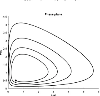
Figure 1.1: The numerical solution of the Lotka–Volterra system with the explicit Euler method, witha=b=1, c=d =0.5,N0= P0 =0.5 andτ=0.1.

The use of the implicit Euler method results in the model N_n+1= N_n+τN_n+1(a−bP_n+1),

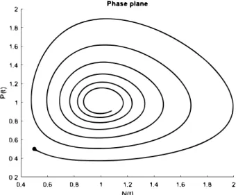
P_n+1= P_n+τP_n+1(cN_n+1−d). (1.25) Figure 1.1 and1.2 suggest that the above methods do not preserve the geometric property, since the numerical solution spirals inwards or outwards, whereas the exact solution should lie on a closed curve.

In the following we define the preservation property of the numerical solution. Let Φτ

represent the mapping of the one-step numerical method

Φτ :y_n→ y_n+1 (1.26)

which, by the analogy with (1.5), we call numerical flow.

Definition 1.16. A numerical method is called symplectic if the one-step mapΦτ is symplectic whenever the method is applied to a smooth Hamiltonian system, i.e.,

Φ⁰_τ(N_n,P_n)^T J Φ⁰_τ(N_n,P_n)= J (1.27) is satisfied.

Definition 1.17. A numerical method is called a Poisson integrator if the numerical flowΦτ

is a Poisson map, i.e., (1.16) holds.

Figure 1.2: The numerical solution of the Lotka–Volterra system with the im- plicit Euler method, with a=b=c=d=1, N₀= P₀=0.5 andτ=0.1.

Hence, we have the following statements.

Theorem 1.18. The explicit Euler and implicit Euler methods are neither symplectic nor Poisson integrators.

Proof. In the following we denote bypⁿandqⁿ the approximations of the unknown functions N(t)andP(t)at the timet =t_n, i.e. N_n = pⁿandP_n=qⁿ, respectively. Applying the explicit Euler method to the Hamiltonian system, we get the following one-step discrete model:











p_n+1 = p_n−τ∂H

∂q(p_n,q_n) q_n+1=q_n+τ∂H

∂p(p_n,q_n).

(1.28)

Therefore,































∂p_n+1

∂p_n =1−τ∂²H

∂q∂p(pn,qn)

∂pn+₁

∂q_n = −τ∂²H

∂q∂q(pn,qn)

∂q_n+1

∂pn

=τ ∂²H

∂p∂p(pn,qn)

∂q_n+1

∂qn

=₁+τ∂²H

∂p∂q(p_n,q_n)_.

(1.29)

From (1.29) by a simple calculation one can check that

(_Φ⁰_τ(p_n,q_n))^TJ(_Φ⁰_τ(p_n,q_n))6= J, (1.30) which means that the explicit Euler method is not a symplectic integrator.

Applying the implicit Euler method to a Hamiltonian system, we get the following one-step numerical method:











p_n+1 = p_n−τ∂H

∂q(p_n+1,q_n+1) q_n+1=q_n+τ∂H

∂p(p_n+1,q_n+1).

(1.31)

We differentiate the above relation with respect top_nandq_n































∂p_n+1

∂pn

=₁−τ∂²H(p_n+1,q_n+1)

∂p∂q

∂p_n+1

∂pn

−τ∂²H(p_n+1,q_n+1)

∂q∂q

∂q_n+1

∂pn

∂p_n+1

∂qn

=−τ∂²H(p_n+1,q_n+1)

∂p∂q

∂p_n+1

∂pn

−τ∂²H(p_n+1,q_n+1)

∂q∂q

∂q_n+1

∂qn

∂q_n+1

∂p_n = τ∂²H(p_n+1,q_n+1)

∂p∂p

∂p_n+1

∂p_n +τ∂²H(p_n+1,q_n+1)

∂q∂q

∂q_n+1

∂p_n

∂q_n+1

∂q_n =1+τ∂²H(p_n+1,q_n+1)

∂p∂p

∂p_n+1

∂p_n +τ∂²H(p_n+1,q_n+1)

∂p∂q

∂q_n+1

∂q_n ,

(1.32)

then the we get again

(_Φ⁰_τ(p_n,q_n))^TJ(_Φ⁰_τ(p_n,q_n))6= J, (1.33) which means that the implicit Euler method is not a symplectic integrator.

Similarly it can be seen that the explicit and implicit Euler methods are not Poisson maps [4,7].

Let us use an explicit-implicit method as follows:

N_n+1= N_n+τN_n+1(a−bP_n),

P_n+1= P_n+τP_n(cN_n+1−d). (1.34) Figure1.3shows the numerical solution of the Lotka–Volterra system with the scheme (1.34).

In this case the numerical result stays on a closed curve.

Figure 1.3: The numerical solution of the Lotka–Volterra system with the sym- plectic Euler method, with a = 0.5, b = 1, c = 0.5, d = 1, N₀ = P₀ = 0.5 andτ=0.1.

Theorem 1.19. The numerical method (1.34) is a symplectic integrator for the transformed Lotka–

Volterra system.

Proof. We apply the above numerical method for the transformed Lotka–Volterra system (1.22) in the following form:

(Nn+₁ = Nn+τ(−be^Pn+a)

P_n+1= P_n+τ(ce^Nn+1 −d) =P_n+τ(e^{Nn+τ(−bePn+a)}−d). (1.35) Differentiating these expressions with respect to N_n andP_n, we get



























∂N_n+1

∂N_n =1

∂Nn+₁

∂Pn

=−be^Pn

∂P_n+1

∂Nn

=τe^{Nn+τ(−bePn+a)}

∂P_n+1

∂P_n =1−be^Pnτe^{Nn+τ(−bePn+a)}.

(1.36)

Hence,

Φ⁰_τ(p_n,q_n)^TJ Φ⁰_τ(p_n,q_n)= J, (1.37) that means the numerical method is a symplectic integrator for the transformed Lotka–

Volterra system. We call this method symplectic Euler method [4].

Theorem 1.20. The symplectic Euler numerical method is a Poisson integrator for the Lotka–Volterra system(1.17).

Proof. From the numerical model (1.34) using some simple calculation, we get

(_Φ⁰_τ(Nn,Pn))^TB(Nn,Pn)(_Φ⁰_τ(Nn,Pn) =B(Nn+₁,Pn+₁) (1.38) with B(Nn,Pn)given in (1.20) and therefore, the method is a Poisson integrator.

The symplectic Euler method, which was analysed in [4,7], is a Poisson integrator and also symplectic for the Lotka–Volterra system. This is the reason why it gives good numerical results. In the next section we combine these methods with the operator splitting method and investigate the geometric properties.

2 Operator splitting methods for the Lotka–Volterra system

The operator splitting method is a powerful tool to lead the time dependent problems to a sequence of simpler sub-problems. This method separates the original equation into two or more parts over a time step, separately computes the solution to each part, and then combines the two or more separate solutions to form an approximation to the solution of the original differential equation. (The generalization for more sub-operators is straightforward, see [3]).

We consider the following Cauchy problem





 dw

dt = A(w(t)) +B(w(t)), 0<t ≤T<_∞ w(0) =w₀,

(2.1)

where w₀ ∈ _R^d is a given vector and the unknown function is w : [0,T) → _R^d. We de- fine a sequence of meshes on the solution domain, with the mesh size τ = ^M_T. We replace the Cauchy problem (2.1) on the above defined M sub-intervals with the following modified Cauchy problems for eachn=1, 2, . . . ,M





 dwⁿ₁

dt (t) =A(wⁿ₁(t)), (n−1)τ<t≤ nτ wⁿ₁((n−1)τ) =wⁿ_sp((n−1)τ),

(2.2)

and 



 dwⁿ₂

dt (t) =B(wⁿ₂(t)), (n−1)τ<t≤ nτ wⁿ₂((n−1)τ) =wⁿ₁(nτ).

(2.3) Here w⁰_sp(0) = w₀, and the function w^M_sp(nτ) = w₂^M(nτ), defined at the points t_n = nτ, (n = 0, 1, . . . ,M) is called splitting solution of the Cauchy problem (2.1). We apply the operator splitting method to the Lotka–Volterra system (1.17) in the following way. Let

V₁(N₁,P₁) =−alnP₁−dlnN₁,

V₂(N₂,P₂) =bP₂+cN₂ (2.4)

a resolution of the functionV. In this case the splitting method leads to the following problems on the interval(n−1)τ<t≤ nτfor eachn =1, 2, . . . ,M:











dN₁ⁿ(t)

dt = aN₁ⁿ(t), N₁ⁿ(tn−1) =N_spⁿ⁻¹ dP₁ⁿ(t)

dt =−dP₁ⁿ(t), P₁ⁿ(t_n−1) =P_spⁿ⁻¹

(2.5)

and 









dN₂ⁿ(t)

dt =−bN₂ⁿ(t)P₂ⁿ(t), N₂ⁿ(t_n−1) = N₁ⁿ(t_n) dP₂ⁿ(t)

dt =cN₂ⁿ(t)P₂ⁿ(t), P₂ⁿ(tn−1) =P₁ⁿ(tn).

(2.6)

(Here the upper indexnrefers to the time interval where the sub-problems are defined.) The above problems can be solved analytically. The first system consists of two separable equations with the exact solution

N₁ⁿ(t) =N_spⁿ⁻¹e^at and P₁ⁿ(t) =P_spⁿ⁻¹e^−dt. (2.7) From the second differential equation, we get

d

dt(cN₂ⁿ+bP₂ⁿ) =0. (2.8)

Therefore cN₂ⁿ+bP₂ⁿ = K₀ is constant, that leads to a Bernoulli-type differential equation.

Hence,

N_spⁿ = ^e

aτN_spⁿ⁻¹K₀ e^K0th

K₀−ce^at·N_spⁿ⁻¹i

+ce^atN_spⁿ⁻¹

(2.9) P_spⁿ = ¹

b h

K₀−cN_spⁿi

, (2.10)

where K₀has the form

K₀=ce^atN_spⁿ⁻¹+be^−dtP_spⁿ⁻¹. (2.11) The flow of the system is the following:

Φt =

"

Φ¹_t(N_spⁿ⁻¹,P_spⁿ⁻¹) Φ²_t(N_spⁿ⁻¹,P_spⁿ⁻¹)

#

, (2.12)

where

Φ¹_t(N_spⁿ⁻¹,P_spⁿ⁻¹):=N_spⁿ and Φ²_t(N_spⁿ⁻¹,P_spⁿ⁻¹):=P_spⁿ. (2.13) With some simple calculation we arrive at the relation

(_Φ⁰_t(N_spⁿ⁻¹,P_spⁿ⁻¹))^TB(N_spⁿ⁻¹,P_spⁿ⁻¹)_Φ⁰_t(N_spⁿ⁻¹,P_spⁿ⁻¹)6= B(N_spⁿ,P_spⁿ)_{, (2.14)} which means the method is not a Poisson integrator.

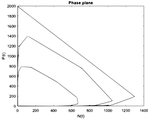
Figure 2.1: The exact solution of system (2.5)–(2.6).

Figure 2.1 shows the exact solutions (2.9) of the systems (2.5)–(2.6). The results show that the solution of the discrete model does not preserve the cyclicity. This is the reason why we use numerical methods to solve both split sub-systems.

We have seen that the explicit Euler and implicit Euler methods in themselves do not preserve the above geometric property. In the sequel, we use the operator splitting method to solve the Lotka–Volterra system (1.17) and using numerical method to the sub-systems. Our expectations for this combined numerical method is that it preserves the geometric properties, namely the symplectic and Poisson structure. In the next sections we will investigate this problem.

2.1 Operator splitting method for a Hamiltonian system

We describe the numerical solution of a Hamiltonian system by using the operator splitting method with given initial conditions. First, we assume that H(p,q) = H₁(p,q) +H₂(p,q)_is some resolution of the Hamiltonian function. Then on each sub-interval[tn,t_n+1]the sequen- tial splitting leads to two sub-problems as follows.









 dp₁

dt =−^∂H1

∂q (p₁(t),q₁(t)) dq₁

dt = ^∂H1

∂p (p₁(t),q₁(t)),

(2.15)

with p₁(tn) =pⁿ_spl andq₁(tn) =qⁿ_spl, and









 dp₂

dt =−^∂H2

∂q (p₂(t),q₂(t)) dq2

dt = ^∂H2

∂p (p₂(t),q₂(t))

(2.16)

with p₂(t_n) = p₁(t_n+1) and q₂(t_n) = q₁(t_n+1). Then we set pⁿ_spl⁺¹ = p₂(t_n+1) and qⁿ_spl⁺¹ = q₂(t_n+1)

We note that although both sub-systems (2.15) and (2.16) are Hamiltonian systems separe- taly, but together they will not Hamiltonian systems anymore in general case.

We apply numerical methods with the step-size equal to the splitting step to these prob- lems and investigate the symplecticity of their flow. We will use the notationspⁿ_i andqⁿ_i for the approximation of the functions p_i(t)andq_i(t)at the mesh-pointt= t_n, respectively (i=1, 2).

We also use the following notations A= ^∂

2H₁

∂p² (pⁿ₁,qⁿ₁), B= ^∂

2H₁

∂q∂p(pⁿ₁,q₁ⁿ), C= ^∂

2H₁

∂q² (pⁿ₁,qⁿ₁), D= ^∂

2H₂

∂p² (pⁿ₂,qⁿ₂), E= ^∂

2H₂

∂p∂q(pⁿ₂,q₂ⁿ), F= ^∂

2H₂

∂q² (pⁿ₂,qⁿ₂).

(2.17)

Then the following statement holds.

Theorem 2.1. By use of the explicit Euler method with a step size equal to the splitting step size to solve the sub-systems(2.15)and(2.16), the combined numerical method is symplectic if the following conditions

ACDF+ACE²−B²DF+B²E²−2BCDE=0 2ACE+2CDE =0 AC−B²+DF−E² =0

(2.18)

are satisfied.

Proof. Applying the explicit Euler method to the sub-problem (2.15) we get











pⁿ₁⁺¹ = p₁ⁿ−τ∂H₁

∂q (pⁿ₁,qⁿ₁) qⁿ₁⁺¹= q₁ⁿ+τ∂H₁

∂p (pⁿ₁,qⁿ₁).

(2.19)

Similarly, the application of the explicit Euler method to the sub-problem (2.16) results in the relation











pⁿ₂⁺¹ = pⁿ₂−τ∂H₂

∂q (pⁿ₂,qⁿ₂) = pⁿ₁⁺¹−τ∂H₂

∂q (pⁿ₁⁺¹,q₁ⁿ⁺¹) qⁿ₂⁺¹=qⁿ₂+τ∂H₂

∂p (pⁿ₂,qⁿ₂) =qⁿ₁⁺¹+τ∂H₂

∂p (p₁ⁿ⁺¹,qⁿ₁⁺¹).

(2.20)

For simplicity, we use the notation pⁿandqⁿfor the approximation of the split solution at the mesh-point t = t_n. Then, the schemes (2.19) and (2.20) together yield the following one-step method











pⁿ⁺¹ = pⁿ−τ∂H₂(pⁿ₁⁺¹,q₁ⁿ⁺¹)

∂q qⁿ⁺¹=qⁿ+τ∂H₂(pⁿ₁⁺¹,q₁ⁿ⁺¹)

∂p ,

(2.21)

where pⁿ₁⁺¹andqⁿ₁⁺¹are defined from (2.19) as follows











pⁿ₁⁺¹ = pⁿ−τ∂H₁

∂q (pⁿ,qⁿ) qⁿ₁⁺¹=qⁿ+τ∂H₁

∂p (pⁿ,qⁿ).

(2.22)

We differentiate these expressions with respect to p andq. Then, according to the chain rule and the notations (2.17), we have

∂pⁿ⁺¹

∂pⁿ = ^∂p

n+1 1

∂pⁿ −τ∂H₂

∂p∂q

∂pⁿ₁⁺¹

∂pⁿ −τ∂H₂

∂²q

∂qⁿ₁⁺¹

∂pⁿ = 1−τB−τE(1−τB)−τ²FA

∂pⁿ⁺¹

∂qⁿ = ^∂p

n+1 1

∂pⁿ −τ∂²H₂

∂q²

∂qⁿ₁⁺¹

∂pⁿ −τ∂²H₂

∂p∂q

∂pⁿ₁⁺¹

∂pⁿ =−τC−τ²CE−τF(₁+τB)

∂qⁿ⁺¹

∂pⁿ = ^∂q

n+1 1

∂pⁿ +τ∂²H₂

∂p²

∂pⁿ₁⁺¹

∂pⁿ +τ∂²H₂

∂p∂q

∂q₁ⁿ⁺¹

∂pⁿ =τA+τD(1−τB) +τ²A

∂qⁿ⁺¹

∂qⁿ = ^∂q

n+1 1

∂qⁿ +τ∂²H₂

∂p²

∂pⁿ₁⁺¹

∂qⁿ +τ∂²H₂

∂p∂q

∂q₁ⁿ⁺¹

∂qⁿ =₁+τB−τ²CD+τE(₁+τB)_.

(2.23)

Hence, computing the matrix product (_Φ⁰_τ(p_n,q_n))^TJ(_Φ⁰_τ(p_n,q_n)) we obtain the sufficient conditions (2.18) for the symplecticity.

This statement shows that the explicit Euler method in itself is not a symplectic integrator, but when we use the operator splitting method with some suitable resolution of the Hamilto- nian function, with such a distribution the method can be symplectic.

The conditions (2.18) are usually very restricitive. Therefore our aim is to relax these con- ditions by choosing other numerical methods for solving the split sub-problems. In the fol- lowing we investigate the combination of the symplectic Euler method and the non-symplectic explicit Euler method. We split the Hamiltonian function into two parts and solve these two sub-systems with the above numerical methods. Let H(p,q) = H₁(p,q) +H₂(p,q) and we solve the first problem with the explicit Euler method











pⁿ₁⁺¹ = pⁿ₁−τ∂H₁(pⁿ₁,q₁ⁿ)

∂q qⁿ₁⁺¹=qⁿ₁+τ∂H₁(pⁿ₁,q₁ⁿ)

∂p ,

(2.24)

then to the second problem we use the symplectic Euler method











pⁿ₂⁺¹= pⁿ₂−τ∂H₂(pⁿ₂⁺¹,qⁿ₂)

∂q ,

qⁿ₂⁺¹ =qⁿ₂+τ∂H2(pⁿ₂⁺¹,qⁿ₂)

∂p .

(2.25)

Theorem 2.2. The combination of the explicit Euler and symplectic Euler method(2.24)–(2.25)results in a symplectic numerical method if the condition

A·B−C=0 (2.26)

is satisfied.

Proof. In the same way, as before to the split porblem (2.15)–(2.16), for this approach the combined method of the explicit and symplectic Euler method can be written as a one-step numerical method, as follows











pⁿ⁺¹ = pⁿ−τ∂H₂(pⁿ⁺¹,qⁿ)

∂q qⁿ⁺¹= qⁿ+τ∂H₂(pⁿ⁺¹,qⁿ)

∂p ,

(2.27)

where pⁿ⁺¹ = pⁿ₂⁺¹, qⁿ⁺¹ = qⁿ₂⁺¹ and qⁿ = qⁿ₁⁺¹. We differentiate these expressions with respect to pⁿ,qⁿ

∂pⁿ⁺¹

∂pⁿ =1−τ∂²H₁(pⁿ₁,q₁ⁿ)

∂p₁∂q₁ −τ∂²H₂(pⁿ⁺¹,qⁿ)

∂p∂q ·^∂p

n+₁

∂pⁿ

−τ²∂²H2(pⁿ⁺¹,qⁿ)

∂q∂q ·^∂

2H₁(p₁ⁿ,qⁿ₁)

∂p₁∂p₁ ,

∂pⁿ⁺¹

∂qⁿ = −τ∂²H₁(pⁿ₁,qⁿ₁)

∂q₁∂q₁ −τ∂²H₂(pⁿ⁺¹,qⁿ)

∂p∂q ·^∂p

n+1

∂qⁿ

−τ∂²H₂(pⁿ⁺¹,qⁿ)

∂q∂q ·

1+τ∂²H₁(pⁿ₁,qⁿ₁)

∂p₁∂q₁

,

∂qⁿ⁺¹

∂pⁿ =τ∂²H₁(pⁿ₁,qⁿ₁)

∂p₁∂p₁ +τ∂²H₂(pⁿ⁺¹,qⁿ)

∂p∂p ·^∂p

n+1

∂pⁿ +τ²∂²H₂(pⁿ⁺¹,qⁿ)

∂p∂q ·^∂

2H₁(p₁ⁿ,qⁿ₁)

∂p₁∂p₁ ,

∂qⁿ⁺¹

∂qⁿ =1+τ∂²H₁(pⁿ₁,q₁ⁿ)

∂p₁∂q₁ +τ∂²H₂(pⁿ⁺¹,qⁿ)

∂p∂p ·^∂p

n+1

∂qⁿ +τ∂²H₂(pⁿ⁺¹,qⁿ)

∂p∂q ·

1+τ∂²H₁(pⁿ₁,qⁿ₁)

∂p₁∂q₁

.

(2.28)

Hence,

(_Φ⁰_τ(p_n,q_n))^TJ(_Φ⁰_τ(p_n,q_n)) =

0 A·B−C+1

−A·B+C−1 0

. Then, by the definition, the numerical method is symplectic if the condition

A·B−C=0 (2.29)

is satisfied.

If we apply these results to the Lotka–Volterra system and choose

H₁=−aP˜₁−dN˜₁ and H2 =be^P˜2 +ce^N˜2, (2.30) the condition of Theorem2.2 is satisfied. In this case the operator splitting has the following biological meaning: the corresponding system has been divided into two terms. The function H₁ shows the growth rate and H₂ contains the interaction terms. Figure 2(a) shows the nu- merical solution with the explicit Euler and symplectic Euler method, when the parameters are a=1,b=0.6,c=0.5,d =1. The solution lies on a closed curve.

We fix these parameters and use the explicit Euler method to solve both systems. We can see that in Figure2(b). In this case the numerical solution spirals outwards.

Let us use the explicit Euler method with another symplectic Euler method and a resolution of the Hamiltonian which does not satisfy the condition of Theorem2.2, namely,

H₁(N^˜₁, ˜P₁) =be^P˜1+ce^N˜1, (2.31) H₂(N^˜₂, ˜P₂) =−aP˜₂−dN˜₂. (2.32) Then the numerical method is not symplectic, see Figure2(c)that shows these cases.

The results show that the adequate combination of numerical methods and splitting meth- ods are useful to preserve the symplectic structure of the numerical solution. As we have seen, the symplecticity depends on the numerical method and the resolution of the Hamilto- nian system, too.

3 Operator splitting method for a Poisson system

We describe the numerical method of the system (1.17) by using the operator splitting method of the form









 dN

dt =−NP·^∂V(N,P)

∂P , N(0) =N0

dP

dt = NP·^∂V(N,P)

∂N , P(0) = P₀.

(3.1)

We investigate the combination of two implicit methods, namely, the implicit Euler method and the symplectic Euler method which results in the sub-problems









 dN₁ⁿ⁺¹

dt =N₁ⁿ−τN₁ⁿ⁺¹P₁ⁿ⁺¹·^∂V1(N₁ⁿ⁺¹P₁ⁿ⁺¹)

∂P₁ , dP₁ⁿ⁺¹

dt = P₁ⁿ+τN₁ⁿ⁺¹P₁ⁿ⁺¹·^∂V1(N₁ⁿ⁺¹,P₁ⁿ⁺¹)

∂N₁ ,

(3.2)









 dN₂ⁿ⁺¹

dt = N₂ⁿ−τN₂ⁿ⁺¹P₂ⁿ·^∂V2(N₂ⁿ⁺¹,P₂ⁿ)

∂P₂ dP₂ⁿ⁺¹

dt =P₂ⁿ+τN₂ⁿ⁺¹P₂ⁿ·^∂V2(N₂ⁿ⁺¹,P₂ⁿ)

∂N₂ .

(3.3)

Theorem 3.1. If we use the combination of the implicit Euler and symplectic Euler method to solve the system(1.17)and the resolution(2.4), then the numerical method is a Poisson integrator.

(a) Numerical solution with the explicit Euler and symplectic Euler method.

(b) Numerical solution with the explicit Euler method.

(c) Numerical solution with the explicit Euler and symplectic Euler method with another resolution of the Hamiltonian system.

Figure 2.2: The numerical solution with the operator splitting method.

Proof. In this case the modified Cauchy problems are the following:

N₁ⁿ⁺¹ = ^N

1n

1−τa, N₁ⁿ =N_spⁿ, P₁ⁿ⁺¹ = ^P

1n

1+τd, P₁ⁿ =P_spⁿ,

(3.4)

and

N₂ⁿ⁺¹ = ^N

2n

1+bτP₂ⁿ, N₂ⁿ= N₁ⁿ⁺¹, P₂ⁿ⁺¹ =P₂ⁿ+τcN₂ⁿ⁺¹P₂ⁿ, P₂ⁿ= P₁ⁿ⁺¹.

(3.5) Hence,











N₂ⁿ⁺¹= (1+τd)N₁ⁿ (1−τa)(1+τd+bτP₁ⁿ) P₂ⁿ⁺¹ = (1+τcN₁ⁿ⁺¹)· ^P

1n

1+τd.

(3.6)

Applying operator splitting and (3.6), we obtain











Nⁿ⁺¹= (1+τd)Nⁿ (1−τa)(1+τd+bτPⁿ) Pⁿ⁺¹ = (1+τcNⁿ⁺¹)· ^P

n

1+τd

(3.7)

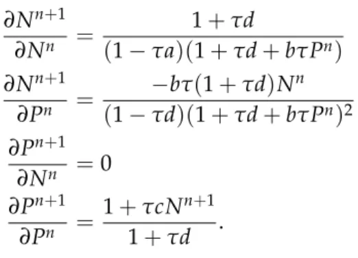
and differentiating these expressions with respect to Nⁿ andPⁿ, we obtain

∂Nⁿ⁺¹

∂Nⁿ = ¹+τd

(₁−τa)(₁+τd+bτPⁿ)

∂Nⁿ⁺¹

∂Pⁿ = −bτ(1+τd)Nⁿ (1−τd)(1+τd+bτPⁿ)²

∂Pⁿ⁺¹

∂Nⁿ =0

∂Pⁿ⁺¹

∂Pⁿ = ¹+τcNⁿ⁺¹ 1+τd .

(3.8)

Therefore, the following condition holds:

(_Φ⁰_τ(Nn,Pn))^TB(Nn,Pn)_Φ⁰_τ(Nn,Pn) =B(N_n+1,P_n+1) (3.9) so the method is a Poisson integrator.

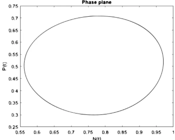
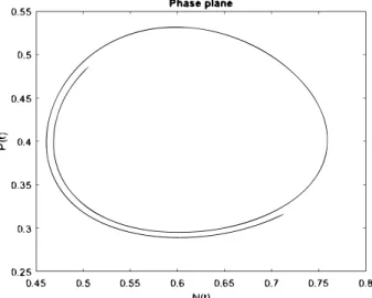
If we chooseV₁ = −alnP−dlnNandV₂ = bP+cN, the numerical method is a Poisson integrator. Figure 3.1 shows the numerical solution with the explicit Euler and symplectic Euler method, when the parameters are a=0.2,b= c=0.5 andd =0.3. The solution lies on a closed curve. We fix these parameters and use the implicit Euler and explicit Euler method

Figure 3.1: Numerical solution with the implicit Euler and symplectic Euler method.

to solve the systems. In this case Figure3.2shows that the numerical solution spirals outward.