Plausible Reasoning in Modular Robotics and Human Reasoning

(1)

Plausible Reasoning in Modular Robotics and Human Reasoning

Claudiu Pozna

University Transilvania of Brasov, Departament of Product Design and Robotics, Bd. Eroilor 28, 500036 Brasov, Romania

E-mail: cp@unitbv.ro

Radu-Emil Precup

Politehnica University of Timisoara, Department of Automation and Applied Informatics, Bd. V. Parvan 2, 300223 Timisoara, Romania

E-mail: radu.precup@aut.upt.ro

Abstract: Present paper continues the researches on cognitive system design. The goal of the paper is to illustrate the variety of models which can be constructed using the Bayesian plausible reasoning theory. The first case study develops a classical inverse kinematical model into a Bayesian model. The second case study models the human reasoning presented by the famous story of Sun Tzu: ‘Advance to Chengang by a hidden path’.

Keywords: model, Bayesian theory, plausible reasoning

1 Introduction

Present paper continues the author’s researches on cognitive system design. These researches have been started by a phenomenological analysis of AI collocation [1]

and have continued by researches on modeling with Bayesian plausible reasoning.

The goal of this paper is to illustrate the variety of phenomenon which can be modeled using the mentioned theory. For this reason we have structured our paper in three parts. The presentation starts with a briefly introduction of the plausible reasoning theoretical background. The second part illustrates the transformation of a classical inverse kinematics problem into a Bayesian model. The third part tried to model a human reasoning example. More precisely, our intention was to explain (by modeling) the famous story of Sun Tzu: ‘Advance to Chengang by a hidden path’.

(2)

The Principles of Plausible Reasoning [6]:

1 The representation of degree of plausibility is given by the plausibility function:

[ ]

0 1 :Φ→

p ; p(A|X)=y (1)

where: Θis a set of sentences;p(A|X) is a continuous and monotonic function which associates a particularly degree of truth for the sentence A in the condition that sentence X is true;

2 The consistence of the commune sense requires the following property for the p function

)

| ( )

|

(AB X p A X p B AX

p = (2)

1 )

| ( )

|

(A X +p ¬A X =

p (3)

)

| ( )

|

(A B X p A X p B X p AB X

p + = + − (4)

n n i

X A

p _i 1 1...

)

|

( = = (5)

where

{ }

Ai |i₌₁_...n is a complete set of mutual excusive sentence Some comments are necessary:

• by consistence we mean:

• every possible way of reasoning a sentence must lead to the same result;

• the equivalent sentences have an equal degree of plausibility;

• in order to obtain the degree of plausibility for a sentence we must take into account all the evidence available;

• p(AB|X) means the plausibility of sentence A and B in the condition that sentence X is true;

• ¬A means non A;

• p(A+B|X) means the plausibility of sentence A or B in the condition that sentence X is true;

Theoretical Results:

Analyzing the mentioned postulates, theoretical results can be deduced. From the beginning we will mention that because the probability function has the same properties (1…5) it can be accepted that the plausibility function is synonymous with the probability function. This is the only reasons that theoretical results from probability theory can be transferred to the theory of plausible reasoning [1].

(3)

We will resume presenting the Bayesian theorem which can easily deduce from (1-5). If we name by d the evidence of an experiment and by hi=1…n a set of mutual exclusive hypotheses the Bayesian theorem tells us that the plausibility of hypothesis hi in the condition of evidence d is equal with the plausibility of hypothesis hi multiplied by the plausibility of evidence d in the condition that hypothesis hi is true and divided by the sum of the same product made for all the hypotheses of the set.

)

| ( ) (

)

| ) (

( )

| (

...

1

k n

k k

i i

i ph pd h

h d h p

p d h

p

∑

=

= (6)

The plausibility of hypothesis hi in the condition of evidence d is named the a posteriori knowledge, the plausibility of hypothesis hi is named the a priori knowledge and the plausibility of evidence d in the condition that hypothesis hi is trough is named the likelihood. The sum from the denominator is named the marginalization sum.

2 The First Case Study: the Robots Inverse Kinematics Problem

There are many methods to solve the inverse kinematics problem. A very good classification of these methods is presented in [2]. The inverse kinematics methods can be divided in:

1 Analytical, which allows the computation of all possible solutions:

a) Closed – form, where the solutions can be expressed as a set a closed – form equations. This method is restricted to a 6 degree of freedom robots;

b) Algebraic elimination based, where the results can be expressed as a solution to a system of multivariable polynomial equations;

2 Numerical, which converge iteratively to a single solution. This solution depends on the initial searching value:

a) Newton – Raphson methods, where the solution is the root of a nonlinear equation. The convergence is slow and is sensitive to robot singularity;

b) Resolved motion rate control method which is an improvement of Newton – Raphson method [3];

c) Methods based on pseudo-inverse computation of the Jacobian, allow the computation for redundant manipulators, cases when the Jacobian is not square [4];

(4)

d) Control theory based methods, which transform the differential equation associated to the inverse kinematics problem in to a control problem [5];

e) Optimizations methods, which transform the problem in to a nonlinear optimization problem [6]

We can add to this list the Artificial Indigence methods. This direction can be exemplified by the Adaptive Neuro-Fuzzy solution presented by MathWorks. All the combinations: joint variables (inputs) – robot gripper positions and orientations (outputs) are computed with the direct kinematics methods. The results of this computation are training data collections. The learning algorithm which, use the training data, tunes the membership functions of a Sugeno-type Fuzzy Inference System using the training input-output data.

From [2] where the mentioned methods are analyzed we know that:

-

The numerical methods can suffer from numerical instability which prevent an algorithm to converge to a solution;

-

The numerical methods have poor reliability near the Jacobian singularities;

-

The numerical methods can be generalized to solve additional constraint and objective function;

-

The analytical method are restricted to 6 degree of freedom system when additional constraint are impose;

-

The Newton–Raphson methods are the slowest and the analytical algorithms are the fastest;

-

The Jacobian transpose method and the optimization method are sensitive to the local minima;

If we analyze the Adaptive – Neuro – Fuzzy solution we can remark the number of computation needed to obtain the training data collection. The proposed method belongs to the Artificial Intelligence and numerical methods because obtaining the inverse kinematics solution will be transformed into a decision problem and these decisions are based on numerical computations [12].

We will start our presentation by the inverse kinematics problem definition. For the robot structure presented in Figure 1 the mentioned problem input is the gripper position and orientation and the solution (output) is the joint variable value.

(5)

Figure 1

The robot structure; the input data P^E and the output data qj

The Problem Definition

The mathematical description of the problem is (7):

∏

⁻

=

= ¹ + 0

1 , m

j j j

E A

P (7)

where: P^E is the homogenous matrix of the robot end point (gripper) position and orientation (the input data); A_j_,_j₊₁ are the homogenous transformation from joint j to joint j+1; m is the joint number.

We mention that matrixesA_j_,_j₊₁depend on the links parameter and also on the joints variable qjwhich are the problem solution (output data). In [10] there are more details on the homogenous matrixes construction when the robot configuration is modular.

Proposed Solution

We will start by mentioning that each actuator has a finite resolution. More precisely there are joint variable which are technical impossible to be realized.

For a 2 degree of freedom (DOF) robot the combination of possible joints variable combination can be expressed with the direct kinematical problem in (8).

j=1 j=2

j=m-1

1 ,

A0 2 ,

A1

m

Am₋₁_,

q1

q2

qm-1

PE

(6)

⎥⎥

⎥

⎦

⎤

⎢⎢

⎢

⎣

⎡

=

⎟⎟

⎟

⎠

⎞

⎜⎜

⎜

⎝

⎛

⎥⎥

⎥

⎦

⎤

⎢⎢

⎢

⎣

⎡ Φ

1 0 0

0

1 1 1 0 0

0

1 1

, 2

, 1

,

, 2 2

, 2 1

, 2

, 1 2

, 1 1

, 1

1 0 2

1 0 1 1 0

1 2 0 2

1 2 0 1 1 2 0

1 1 0 2

1 1 0 1 1 1 0

) , ( . ) , ( ) , (

. . . .

) , ( . ) , ( ) , (

. . . .

) , ( . ) , ( ) , (

n n n

n

n n n n n

n

n n

y x y

x y x

y x y

x y x

y x y

x y x

q q q

(8)

where: Φis an operator which transforms the joint variable into the robot end point position.

The consequence of this observation is that there are positions of the robot end point which are technical impossible to be obtained by the robot and in these cases the only solution is to approximate them. The generalization of this observation means that for each desired position and orientation of the robot end point we must obtain a suitable combination of the joint variable. This combination will lead to an approximation of the desired position and orientation.

If we resume to the end point position, the approximation means that the distance between the robot end point (x,y,z)_i₁_,_i₂_,..._i_m₋₁ and the desired point (input of the inverse kinematics problem) must accomplish the following condition.

(

x y z _i _i _i ₋ x y z _D

)

≤ρ

d ( , , )₀_,₂_,...m₁,( , , ) (9)

where: ρis the approximation distance, this means the radius of the desired point vicinity inside which the approximation is accepted (see Figure 2); i0,…im-1 are the joint variable index, m is the number of joints.

Figure 2

The desired point approximation

It is clear that we can transform the condition (9) into an optimization problem (10). In this case the appropriate combination of angle is the combination which minimizes the distance between the desired point and robot end point.

( )

(

i i i D

)

n

i d x y z x yz

i m k

) , , ( , ) , , (

min ₀_,₂_,... ₁

...

1 ⁻

∈ (10)

ρ (x,y,z)D

(x,y,z)i1…im

(7)

From this point of view the inverse kinematics problem can be transformed into a search problem. By searching we will analyze the joints variables combinations.

More precisely the mentioned combinations will be transformed by direct kinematics method in to the robot end point positions, and then these positions will be used in (9) or (10). For this problem we must find a method which:

• Decreases the number of searching steps;

• Avoids the search divergence.

Our idea starts from this point. The proposed searching algorithm will be managed by the plausible reasoning theory. In order to do this we will use the Bayesian theorem. We will rewrite the mentioned theorem:

)

| ( ) ( )

|

(h_i⁺^,⁻ o ∝ p h_i⁺^,⁻ p o h_i⁺^,⁻

p (11)

where: “h_i^+,⁻”is the sentence: “In order to obtain (9) the joint variable from joint i must be increased, (decreased)”; “o” is the observation of approximation in term of (9) when the action of increasing (decreasing) tack place; ∝ means proportional; i=0...m−1is the current number of joints.

Some comments are necessary:

• Searching the appropriate combination for a desired point means an iterative process;

• The plausibility p(h_i⁺^,−) is an a priori known: for the initial step of the iteration we have no knowledge in order to consider one sentence more plausible the other. This means that all the sentence have the same plausibility;

• Usually the likelihood p(o|h_i⁺^,−) is an a priori knowledge, in this case we must compute, by direct kinematics method, the position of the robot end point and to compare this value with de desired point. Therefore we have defined the likelihood by (12):

) ) , , ( , ) , , ((

) 1

| (

1 2 0, ,...

,

D i

i i

i d x y z x y z

h o p

m−

− =

+ (12)

• The a posteriori plausibility p(h_i⁺^,⁻|o)will be obtained by normalizing (11).

In the next iteration step this plausibility will become the a priori plausibility;

• At each step (epoch) we must compute p(h_i⁺^,⁻|o) these means 2xm plausibility computation. From this set we will choose the sentence which has the maximum plausibility and we will perform the increasing (decreasing) mentioned in this sentence;

(8)

• In order to avoid the searching divergence we will impose a maximum number of epochs. If condition (9) is accomplished, the searching algorithm will end. If not, the algorithm will perform the maximum number of epochs and will output the joints variables which lead to the minimum distance between the desired point and the robot end point;

• A possible divergence cause is the fact that all possible end points are out from the vicinity of the desired point (see Figure 3). For this situation usually we say that the desired point is out of the working volume. Actually we deal with a set of possible points ‘points cloud’. These points intersects or not the mentioned vicinity;

Figure 3

The desired point is out of the points cloud

• A desired trajectory is a set of desired points. The algorithm performs searching for each desired point and output the joints variables. Performing the direct kinematics for these joints variable we will obtain a trajectory which approximate the desired trajectory;

• In order to increase the smooth of the approximation we have develop our algorithm by introducing a dynamic vicinity of the desired points. More precisely if the algorithm converges for radius ρi we will perform a new search for radius ρ_i+1=0.5 ρ_i. The dynamic vicinity search will end when a divergence occurs or when the radius is smaller than an imposed value, this means ρk<ρmin.

The Algorithm

If we summarize these considerations we can propose the following algorithm for the inverse kinematics problem:

1 The initial (input) data are:

• the robot configuration, here this means the necessary data for compute the homogenous transformations (A_j_,_j₊₁);

• the robot resolution for each joint (Δ0…m-1);

• the approximation radius (ρ);

ρ

(x,y,z)D

(x,y,z)i1…im

(9)

• the initial position of the robot (q0…m-1);

• a set of desired points (x,y,z)D0…r;

• the epochs number (Nepochs);

2 For each desired point a searching algorithm can have Nepochs, and start with:

• setting the a priori plausibility: p(h_i⁺^,−)=1/2m, i=0…m-1;

3 The searching algorithms epoch means:

• computing the likelihood by (12), for all 2xm sentences; the end point position is computed by (1) for q_i=q_i±Δ_i;

• computing the a posterior plausibility with (11) for each 2xm sentences;

• finding the maximum plausibility ( | ) max ( ^, | )

...

1

, o p h o

h

p _i

m k i

− +

=

−

+ = ;

• set the angel values: q_i=q_i;i=0...m−1;i≠k q_k =q_k±Δ_k;

• set the a priori plausibility: p(h_i⁺^,⁻)= p(h_i⁺^,⁻|o);

• if condition (9) is accomplished then:

• set q_i^S_,_j=q_i where q_i^S_,_j means the solution for joint i at the desired point j;i=0...m−1;j=0...r;

• go to the next desired point;

• if condition (9) is not accomplished then

• setq_i^PS^,^k =q_i; d^k =d;q_i^PS^,^kmeans the possible solution at epoch k , k=1… Nepochs

• start a new searching epoch;

4 If after Nepochs the condition (9) is not accomplished then set q_i^S_,_j =q_i^PS^,^l where

epochs N k

k

l d

d

...

1 )

min(=

= ;

5 In the end the problem solution (output) consists on a set of angular values for each desired point:

{

, ^| =⁰^... ^; =⁰^... −¹

}

= q j r i m

Q _i^S_j

In the next section results simulation of the proposed algorithm are presented.

(10)

The Simulations

The proposed algorithm was transformed into a computer program. We have used this program for several robots configurations (several DOF) and several desired trajectories.

After obtaining the inverse kinematics solution the program animates the robot for each desired point. In this way we have observed the continuity of the robots movements.

In the simulation we have used Δi=0.005[rad]; ρ=3[mm]; NEpochs=100;

Figure 4

Simulation for a 2 DOF robot

Figure 5

Simulation for a 3 DOF robot

Figure 6

Simulation for a circlular desired trajectory

Figure 7

Simulation for a sloping desired trajectory

In Figure 4 a 2DOF robot which performs a horizontal trajectory is presented. In Figure 5 a 3 DOF robot performs a vertical trajectory. This trajectory starts at (1.7,0) goes to (1.7,-1.7) returns at the first point and end at (1.7,1.69).

(11)

Figure 8

Simulation for a parabolic desired trajectory

Figure 9 An epoch: the convergence

In Figure 6, 7 and 8 the 3DOF robot performs a circular, sloping, respectively a parabolic trajectory. In the end, in Figure 9 the convergence processes is presented. More precisely the robot joints variables starting point is marked with

“o” and during an epoch these variables converges to the final joints variables, marked by the arrow. The final joints variables are the solutions q_i^S_,_j and will be memories in the problem solution set.

Conclusions

Present work continues the research program, about the modular robots by proposing a new solution for the inverse kinematics problem. This is a numerical solution based in plausible reasoning theory that is the Bayesian theorem. The mentioned theorem was adapted for a searching algorithm in order to obtain an accepted approximation of the desired robot end point.

The proposed solution’s limitations are that we haven’t considered the possible conditions (avoiding obstacles etc.) and the fact that the solution depends on the initial values. In future works we intend to generalize the method for optimization problems and also to replace the desired points (xyz) position by the analytical form of the desired trajectory.

3 The Second Case Study: a Strategically Problem

The intention of the third case study is to prouve the ability of Plausible Reasoning in human reasoning modeling. For this pourpouse we will tray to model the famous story of Sun Tzu: ‘Advance to Chencang by a hidden path’.

The story that we intend to explain by Bayesian model is the following:

This stratagem took place towards the end of the Qin dynasty. Xiang Yu appointed Liu Bang as king of Hanzhong, effectively making him leave China. To further ensure that Liu Bang does not return to China from the East, Xiang Yu divided

(12)

Guanzhong into three principalities and put three people in charge, informing them to be alert against Liu Bang.

Liu Bang said, ‘In order to placate Xiang Yu and the three kings, we must destroy the mountain plank road to show that we've no intention of returning to China.’

After nine years of preparations, Liu Bang's army became powerful and was ready to march eastwards. Liu Bang ordered his generals to take 10,000 men and horses and repair the plank road within three months.

Meanwhile, his enemies were greatly perturbed. One of the kings even led his forces to block the plank road exit.

Liu Bang then led his generals and several thousand troops to overrun Guanzhong by the old roundabout route through Chencang.

We intend to model this story by using the Bayesian theorem (6). At first sight the victory of Liu Bang is based on his ability to increase the plausibility of the likelihood that he will attack on the plank road.

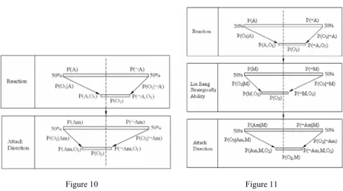
If we analyze more deeply the story we will find that there are two stage of the conflict: the first when Liu Bang must decide about the reaction concerning the Xiang Yu actions, and the second when Liu Bang shows his attack intention but he must choose the attack direction.The story scenario is presented in Figure 10. It can be see that in the first stage of the conflict, by destroying the road Liu Bang have increased the peace (non attack) likelihood and in this way manipulate Xiang You. In the second stage of the conflict by restoring the road Liu Bang have increased the mountain direction attack (Am) and manipulate once again his enemy. From mathematical point of view this scenario can be describe in the following way:

• in the initial moment Xiang You can not decide the intention of Liu Bang:

o P(A)=P(¬A)=50%; where A is the sentence ‘Liu Bang will attack’

• after seeing that Liu Bang destroyed the road Xiang You decides that:

o P(O₁|¬A)>P(O₁|A); where O1 is the observation of the destroyed road;

o in consequence (6) P(¬A|O₁)>P(A|O₁);

• in the initial moment Xiang You can not decide the attack direction of Liu Bang:

o P(Am)=P(¬Am)=50%; where Am is the sentence ‘Liu Bang will attack from the mountain’;

• after seeing that Liu Bang constructs the road Xiang You decides that:

(13)

o P(O₂|Am)>P(O₂|¬Am); where O2 is the observation of the constructed road;

o in consequence (6) P(Am|O₂)>P(¬Am|O₂)

Figure 10 The story scenari

Figure 11 A posible solution

The famous story can be continued with a problem: have had Xiuag You the chance to react at his opponent ability? There are several solutions of this problem the first consist on increasing the number of hypothesis of attack direction and find new observations (spy). The second solution is presented in Figure 11 and is based on changing the causal network by introducing a new decision step. More precisely it can be see that after the second observation O2 Xiuang You becomes able to decide the tactic that Liu Bang will use. This observation increases the likelihood that his opponent uses his ability to manipulate him.

From mathematical point of view this solution can be described in the following way:

• in the initial moment Xiang You can not decide the intention of Liu Bang:

o P(A)=P(¬A)=50%; where A is the sentence ‘Liu Bang will attack’

• after seeing that Liu Bang destroyed the road Xiang You decides that:

o P(O₁|¬A)>P(O₁|A); where O1 is the observation of the destroyed road;

o in consequence (6) P(¬A|O₁)>P(A|O₁);

• in the initial moment Xiang You can not decide about the strategically ability of his opponent:

(14)

o P(M)=P(¬M)=50%; where M is the sentence ‘Liu Bang is able to manipulete’

• after seeing that Liu Bang intends to attack Xiang You decides that:

o P(O₂|M)>P(O₂|¬M); where O2 is the observation of the constructed road; M is the sentence ‘Liu Bang is able to manipulate’

o in consequence (6) P(M |O₂)>P(¬M |O₂);

• in the initial moment Xiang You can not decide the attack direction of Liu Bang:

o P(Am)=P(¬Am)=50%; where Am is the sentence ‘Liu Bang will attack from the mountain’;

• after seeing that Liu Bang constructs the road, and knowing that his opponent can manipulate Xiang You decide that:

o P(O₂|Am,M)<P(O₂|¬Am,M);

o in consequence (6) P(Am|O₂,M)<P(¬Am|O₂,M) Conclusions

The second case study illustrates the ability of the plausible reasoning in modeling the human reasoning. It was presented the analysis of a famous strategically story and the synthesis of a problem. New solutions obtained by developing the causal network are very attractive.

4 Final Conclusions

Present paper continues the author researches on cognition system design by presenting two different case studies which use the same theory: the Bayesian theory of plausible reasoning. The first case study develops classical inverse kinematics problems in to a Bayesian model by proposing a searching algorithm.

In the second case study end we have tray to model by Bayesian theory one of the famous stories of Sun Tzu.

Acknowledgement

This research work is supported by the Romanian Ministry of Education and Research trough CNCSIS project 895/2007.

(15)

References

[1] C. Pozna, A Phenomenological Analysis Trial of the AI syntagma, In Proceedings of the 7^th International Symposium of Hungarian Researchers, Budapest 2006, pp. 159-165

[2] D. Tolani, A. Goswami, N. I. Badler, Real-Time Inverse Kinematics Techniques for Anthropomorphic Limbs Graphical Models 62(5): pp. 353- 388, 2000

[3] D. E. Whitney, Resolved Motion Rate Control of Manipulators and Human Prostheses, IEEE Trans. Man–Machine Systems 10, pp. 47-63, 1969 [4] C. Klein, C. Huang, Review of Pseudoinverse Control for Use with

Kinematically Redundant Manipulators, IEEE Trans. Systems Man Cybernet. 7, pp. 868-871, 1997

[5] L. Sciavicco, B. Siciliano, Modeling and Control of Robot Manipulators, McGraw–Hill, NewYork, 1996

[6] J. Zhao, N. Badler, Inverse Kinematics Positioning Using Nonlinear Programming for Highly Articulated Figures, Trans. Comput. Graph.

13(4), pp. 313-336, 1994

[7] Jaynes, E. T., Probability Theory with Application in Science and Engineering, Washington University, 1974

[8] http://yudkowsky.net/bayes/bayes.html Yudkowsky, E., An Intuitive Explanation of Bayesian Reasoning

[9] J. Pearl. Causality: Models, Reasoning, and Inference, Cambridge Univ.

Press, New York, 2000

[10] C. Pozna, Modular Robots Kinematics, Journal of Applied Science at Budapest Tech, Vol. 3, Nr. 2, pp. 5-18, 2007

[11] Rudas, I., Evolutionary Operators New Parametric Type Operators Family, Fuzzy Sets and Systems 23, pp. 149-166