Constrained Predictive Control of Three- PhaseBuck Rectifiers
László Richárd Neukirchner
1, Attila Magyar
1, Attila Fodor
1, Nimród Dénes Kutasi
2, András Kelemen
21 University of Pannonia, Department of Information Technology, Egyetem u. 10, 8200 Veszprém, Hungary, e-mails: neukirchner.laszlo@virt.uni-pannon.hu, magyar.attila@virt.uni-pannon.hu, foa@almos.uni-pannon.hu
2 Sapientia Hungarian University of Transylvania, Department of Electrical Engineering, Corunca 540485, Romania, e-mail: kutasi@ms.sapientia.ro, kandras@ms.sapientia.ro
Abstract: In this paper, constrained optimal control of a current source rectifier (CSR) is presented, based on a mathematical model developed in Park’s frame. To comply with the system constraints an explicit model-based predictive controller was established. To simplify the control design, and avoid linearization, a disjointed model was utilised due to the significant time constant differences between the AC and DC side dynamics. As a result, active damping was used on the AC side, and explicit Model Predictive Control (MPC) on the DC side, avoiding non-linear dynamics. The results are compared by simulation with the performance of a state feedback control.
Keywords: model predictive control; current source rectifier; space vector modulation;
modeling; constrained control
1 Introduction
Current source rectifiers (CSR) are widely used in front-end power electronic converter for the uncontrollable or controllable DC-bus in industrial and commercial applications. They have maintained their position through many applications, with uses such as medium-voltage high-power drives [1], [2]
STATCOMs [3] and renewable systems [4], [5]. They have a plain and reliable circuit structure, which makes them attractive for simple control design. The CSRs are traditionally controlled by classic cascaded linear control loops such as PI controllers. These simple control applications are suitable for induction motor control [6], and other electromechanical actuators [7], and unusual topologies [8].
Also, worth mentioning is self-tuning variants of PI controllers [9]. In the past, the modulation methods used were trapezoidal pulse width modulation techniques
(TPWM), or application of pulse patterns calculated offline for selective harmonic elimination (SHE). More recently, current space vector modulation (SVM) has been used for the synthesis of the transistor control signals [10]. Even so, AC-side harmonic elimination could still be an issue at lower switching frequencies where LCL filtering would be advised [11]. In order to keep switching frequencies low and to minimize switching losses, new topologies and hybrid modulations are used, mixing TPWM and SHE depending on the grid frequency [12].
In terms of the amplitude of the grid and DC-link voltages, CSRs exhibit a step- down conversion. When used as DC voltage source, the rectifier can output a lower DC voltage without the need of a grid-side transformer, as is usually employed in voltage source rectifiers (VSR). Because of their current source behaviour, CSRs can be easily paralleled and provide inherent short-circuit protection, representing an excellent potential in DC power supply applications [13], [14].
There are several control strategies in addition to classical PI control for applications in this domain. Self-adapting control methods are on the rise with more sophisticated algorithms in the field of fuzzy logic [15]. They are capable of handling increasingly more complicated models and systems with high dynamics and accuracy [16], [17], and even without establishing and validating classical state-space models [18]. The other filed is the sliding mode control, which can achieve good dynamic performance and handle non-linearity. Still, they might also introduce chattering, which can be very undesirable when applied to real-life systems like in [19] and [20].
In the linear domain implicit model predictive control (IMPC or just MPC) is a fair solution due its; effectiveness in power electronics, configurable cost function and such scalable nature [21], [22]. In this field also finite-state solutions are present which can be considered also predictive control, where the modulation scheme’s defined states serve as optimization potential [23], [24]. As a further step adaptive application was established to tackle parameter estimation problems for better performance [25]
Recently, beside implicit, finite-state, and adaptive predictive control, explicit model predictive control has emerged in the field of power electronics [26].
Establishing the MPC cost function can range widely depending on the expected dynamics, degree of noise cancellation, and model complexity. Additionally, the current limitation can also be implemented introducing constraints in the modulation algorithm.
In [27] the validity of an MPC-based, digital pulse width modulation control strategy for single-phase voltage source rectifiers is discussed, further confirming the validity of this method in control systems.
1.1 New Contributions
In this paper a model predictive control method is developed for a classical current source buck-type rectifier (CSR). The contribution of the paper is to show how to design EMPC on a model of a CSR which has a complex model due to bilinearity.
To overcome the burden of bilinearity a simple solution is shown which enables handling the model parts as linear disjointed systems of their own.
The structure of the paper is as follows. In Section 2 the topology is presented, followed by the mathematical model derived in the synchronous rotating coordinate frame. Next, the control structure is presented, followed by the detailed description of the DC-side Explicit Model Predictive Control (EMPC) and by the presentation of the AC-side active damping. In the fourth section, the current space vector modulation scheme is shown, with optimized switching pattern to reduce the switching frequency. Lastly, the simulation results are presented and the performance of the proposed control structure is compared with the performance of a state feedback controller, before the conclusions are finally drawn.
2 Mathematical Modeling of the CSR
The structure of the classical three phase buck-type current source rectifier (CSR) is presented in Fig. 1. In continuous current mode, the differential equations corresponding to the CRS’s inductor currents and capacitor voltages are the following:
Figure 1
Circuit diagram of the three-phase buck-type rectifier with insulated gate bipolar transistors (IGBTs)
𝐿𝑎𝑐𝑖𝑎𝑐̇ = 𝑢𝑝 𝑝− 𝑢𝑐𝑝− 𝑅𝑖𝑎𝑐𝑝 (1)
𝐶𝑎𝑐𝑢𝑐̇ = 𝑖𝑝 𝑎𝑐𝑝− 𝛿𝑝𝑖𝑑𝑐 𝐿𝑑𝑐𝑖𝑑𝑐̇ = (∑ 𝛿𝑝
3
𝑝=1
𝑢𝑐𝑝) − 𝑢0
𝐶𝑑𝑐𝑢0̇ = 𝑖𝑑𝑐− 𝑢0
𝑅𝑙𝑜𝑎𝑑
where 𝑝 ∈ {1, 2,3} is the index of three phases and 𝛿𝑝 describes the conduction state of the rectifier leg 𝑝 (2).
𝛿𝑝= {
1 𝑖𝑓 𝑡ℎ𝑒 𝑢𝑝𝑝𝑒𝑟 𝑡𝑟𝑎𝑛𝑠𝑖𝑡𝑜𝑟 𝑖𝑠 𝑂𝑁
−1 𝑖𝑓 𝑡ℎ𝑒 𝑙𝑜𝑤𝑒𝑟 𝑡𝑟𝑎𝑛𝑠𝑖𝑠𝑡𝑜𝑟 𝑖𝑠 𝑂𝑁 0 𝑖𝑓 𝑏𝑜𝑡ℎ 𝑎𝑟𝑒 𝑂𝑁 𝑜𝑟 𝑂𝐹𝐹
(2)
Using the components in the stationary frame of the space phasors of the three- phase quantities, from (1) it results:
𝐿𝑎𝑐𝑖𝑎𝑐̇ = 𝑢𝛼 𝛼− 𝑢𝑐𝛼− 𝑅𝑖𝑎𝑐𝛼 𝐿𝑎𝑐𝑖𝑎𝑐̇ = 𝑢𝛽 𝛽− 𝑢𝑐𝛽− 𝑅𝑖𝑎𝑐𝛽 𝐶𝑎𝑐𝑢𝑐̇ = 𝑖𝛼 𝑎𝑐𝛼− 𝛿𝛼𝑖𝑑𝑐
𝐶𝑎𝑐𝑢𝑐̇ = 𝑖𝛽 𝑎𝑐𝛽− 𝛿𝛽𝑖𝑞𝑐
𝐿𝑑𝑐𝑖𝑑𝑐̇ = 1.5 (𝛿𝛼𝑢𝑐𝛼+ 𝛿𝛽𝑢𝑐𝛽) − 𝑢0
𝐶𝑑𝑐𝑢0̇ = 𝑖𝑑𝑐− 𝑢0 𝑅𝑙𝑜𝑎𝑑
(3)
Equation (3) is transformed to the synchronous reference frame rotating with the 𝑢𝑐𝑑 capacitor voltage space vector. The resulting mathematical model is thus:
𝐿𝑎𝑐𝑖𝑎𝑐̇ = 𝑢𝑑 𝑑− 𝑢𝑐𝑑− 𝑅i𝑎𝑐𝑑+ 𝜔𝑠𝐿𝑎𝑐i𝑎𝑐𝑞
𝐿𝑎𝑐𝑖𝑎𝑐̇ = 𝑢𝑞 𝑞− 𝑢𝑐𝑞− 𝑅i𝑎𝑐𝑞− 𝜔𝑠𝐿𝑎𝑐i𝑎𝑐𝑑 𝐶𝑎𝑐𝑢𝑐̇ = 𝑖𝑑 𝑎𝑐𝑑− 𝛿𝑑𝑖𝑑𝑐+ 𝜔𝑠𝐶𝑎𝑐𝑢𝑐𝑞
𝐶𝑎𝑐𝑢𝑐̇ = 𝑖𝑞 𝑎𝑐𝑞− 𝛿𝑞𝑖𝑑𝑐− 𝜔𝑠𝐶𝑎𝑐𝑢𝑐𝑑
𝐿𝑑𝑐𝑖𝑑𝑐̇ = 1.5 (𝛿𝑑𝑢𝑐𝑑+ 𝛿𝑞𝑢𝑐𝑞) − 𝑢0
𝐶𝑑𝑐𝑢0̇ = 𝑖𝑑𝑐− 𝑢0 𝑅𝑙𝑜𝑎𝑑
where 𝜔𝑠 represents the network voltage vector’s angular velocity.
(4)
2.1 Model Simplification
Notice, that the sixth-order ODE model (4) is bilinear in its states and inputs because of the product terms (𝛿𝑑𝑖𝑑𝑐 for example). As such, using design methods for linear systems is not straightforward. The high complexity given by the system’s order is another problem to tackle. For designing classic MPC, linear, low-order equation systems are favorable. Hence
simplification of the model would bring noteworthy benefits, making the MPC design more straightforward, when a linear system resulted.
Since the AC and DC side’s time constants differ significantly (as in the AC: 𝜔𝑎𝑐=√𝐿1
𝑎𝑐𝐶𝑎𝑐≅ 5.7 ∙ 103[𝑟𝑎𝑑/𝑠], and on the DC:𝜔𝑑𝑐 = 1
√𝐿𝑑𝑐𝐶𝑑𝑐≅ 2.8 ∙ 102[𝑟𝑎𝑑/𝑠], see Table 3. for reference). Thus, the differential equations can be separated into two sets, and the control of the AC and DC sides can be decoupled as described in [28]. The AC side model results as follows:
( 𝑖𝑎𝑐̇𝑑 𝑖𝑎𝑐̇𝑞 𝑢𝑐̇𝑑 𝑢𝑐̇𝑞)
=
(
− 𝑅
𝐿𝑎𝑐 𝜔𝑠 − 1 𝐿𝑎𝑐 0
−𝜔𝑠 − 𝑅
𝐿𝑎𝑐 0 − 1
𝐿𝑎𝑐 1
𝐶𝑎𝑐 0 0 𝜔𝑠
0 1
𝐶𝑎𝑐 −𝜔𝑠 0
) (
𝑖𝑎𝑐𝑑 𝑖𝑎𝑐𝑞 𝑢𝑐𝑑 𝑢𝑐𝑞)
+
( 𝑢𝑑 𝐿𝑎𝑐 𝑢𝑞 𝐿𝑎𝑐
−𝛿𝑑𝑖𝑑𝑐 𝐶𝑎𝑐
−𝛿𝑞𝑖𝑑𝑐 𝐶𝑎𝑐 )
. (5)
Looking at the state matrix it can be further stated that there are only weak couplings between the 𝑑 and 𝑞 components. This allows to handle them separately, and later to design separate control for each.
The equation system describing the DC side dynamics is the following:
(𝑖𝑑𝑐̇ 𝑢0̇ ) = (
0 𝐿−1
1 𝑑𝑐 𝐶𝑑𝑐
−1 𝑅𝑙𝑜𝑎𝑑𝐶𝑑𝑐
) (𝑖𝑑𝑐
𝑢0) + (
1.5
𝐿𝑑𝑐(𝛿𝑑𝑢𝑐𝑑+ 𝛿𝑞𝑢𝑐𝑞)
0 ). (6)
It can be noticed that, with the AC and DC model separation, bilinearity disappears, since the binding coefficients are present only in the input (𝒖) of the DC state space model. Consequently, all equations are linear and with a considerably lower order, making control design much easier and allowing for the application of linear design methods. For the DC side dynamics, the linear time invariant differential equation system’s matrices can be identified for predictive control design purposes:
𝒙 = (𝑖𝑑𝑐
𝑢0) , 𝒖 = (𝛿𝑑𝑢𝑐𝑑+ 𝛿𝑞𝑢𝑐𝑞) , 𝒚 = 𝑢0, 𝑨 = (0 𝐿−1
1 𝑑𝑐 𝐶𝑑𝑐
−1 𝑅𝑙𝑜𝑎𝑑𝐶𝑑𝑐
) , 𝑩 = (
1.5 𝐿𝑑𝑐
0) , 𝑪 = (0 1).
(7)
where 𝒙, 𝒖and 𝒚are the state, input and output vectors of the DC-side system, and A, B and C are the state, input and output matrices.
The circuit parameters used for the implementation of the control structure based on this model are presented in Table 3.
3 The Control Structure
Relying on the possibility of separation of the AC-side and DC-side controllers, the control structure from Fig. 2 is proposed.
Figure 2
Block diagram of the control structure
The controllers operate in the synchronous frame of the AC filter capacitor voltages 𝑢𝑐(1,2,3), and the rectifier input currents 𝑖𝑟(1,2,3) are in phase with the capacitor voltages.
The current reference 𝑖𝑟(𝛼𝛽)∗ supplied to the space vector modulation unit in the stationary frame, is obtained by coordinate transformation [𝐷(−𝜃)] of the current reference (8) delivered by the current controllers in the synchronous frame.
{𝑖𝑟∗𝑑= 𝑖𝑟𝑐𝑜𝑛𝑡𝑟𝑜𝑙𝑑+ 𝑖𝑟𝐻𝐹𝑑
𝑖𝑟∗𝑞= 0 (8)
In (8), 𝑖𝑟𝑐𝑜𝑛𝑡𝑟𝑜𝑙𝑑 represents the output of the DC voltage controller, while 𝑖𝑟𝐻𝐹𝑑 represents the damping current, proportional with the high frequency component of the filter capacitor voltage (the fundamental component of the capacitor voltage in the stationary frame becomes a DC component in the synchronous frame). The DC and AC side control units are explained in more detail in the following sections, and the performance of the control structure is evaluated.
3.1 DC-SideExplicit Model Predictive Control
Model predictive control (MPC) is an efficient and systematic method for solving complex multi-variable constrained optimal control problems [3]. The MPC control law is based on the “receding horizon formulation”, where the model’s assumed behavior is calculated for a number of 𝑁 steps, where N stands for the
horizon’s length. Only the first step of the computed optimal input is applied in each iteration. The remaining steps of the optimal control input are discarded and a new optimal control problem is solved at the next sample time. Using this approach, the receding horizon policy provides the controller with the desired feedback characteristics, although with high order systems the computational effort is considerably demanding since all the steps should be taken in to account on the specified horizon in every iteration. With Explicit MPC (EMPC), the discrete time constrained optimal control problem is reformulated as multi- parametric linear or quadratic programming. Using this approach, the problem of optimization can be solved offline, making it much more feasible from the perspective of the optimal control task. The optimum control law is a piecewise affine function of the states, and the resulting solution is stored in a pre-calculated lookup table. The parameter space, or the state-space is partitioned into critical regions. The real-time implementation consists in searching for the active critical region, where the measured state variables lie, and in applying the corresponding piecewise affine control law to achieve the desired dynamics.
In order to introduce the MPC implementation from this paper, let us consider a linear discrete time system (9) derived with the discretisation of system (6) with zero-order hold method, where control inputs are assumed piecewise constant over the simulation sample time 𝑇𝑠= 1 𝑓⁄ 𝑠:
𝒙(𝑡 + 1) = 𝑨𝑑𝒙(𝑡) + 𝑩𝑑𝒖(𝑡)
𝒚(𝑡) = 𝑪𝑑𝒙(𝑡) (9)
where 𝑨𝑑, 𝑩𝑑, 𝑪𝑑ere the matrices of the discretised system derived from (7). With system (9) appears to be linear time invariant, MPC design can be followed. The following constraints have to be satisfied:
𝒚𝑚𝑖𝑛≤ 𝒚(𝑡) ≤ 𝐲𝑚𝑎𝑥, 𝒖𝑚𝑖𝑛 ≤ 𝒖(𝑡) ≤ 𝒖𝑚𝑎𝑥 (10) where 𝑡 > 0, 𝒙 ∈ 𝑅𝑛, 𝒖 ∈ 𝑅𝑚, 𝒚 ∈ 𝑅𝑝. The MPC solves the following constrained optimization problem [23]:
𝑈={𝒖𝑡,…,𝒖𝑚𝑖𝑛𝑡+𝑁𝑢−1}𝐽(𝒖, 𝒙(𝑡)) = ∑ (𝒙𝑡+𝑁𝑇 𝑦∨𝑡𝑄𝑤𝒙𝑡+𝑁𝑦∨𝑡+ 𝒖𝑡+𝑘𝑇 𝑅𝑤𝒖𝑡+𝑘)
𝑁𝑦−1
𝑘=0
(11) subject to:
𝒙𝑚𝑖𝑛 ≤ 𝒙𝑡+𝑘|𝑡 ≤ 𝒙𝑚𝑎𝑥, 𝑘 = 1, … , 𝑁𝑐− 1 𝒖𝑚𝑖𝑛 ≤ 𝒖𝑡+𝑘|𝑡 ≤ 𝒖𝑚𝑎𝑥, 𝑘 = 0,1, … , 𝑁𝑐− 1 𝒙𝑡|𝑡= 𝒙
(
𝑡)
𝒙𝑡+𝑘+1|𝑡 = 𝑨𝑑𝒙𝑡+𝑘|𝑡+ 𝑩𝑑𝒖𝑡+𝑘|𝑢 𝒚𝑡+𝑘+1|𝑡 = 𝑪𝑑𝑥𝑡+𝑘|𝑡
𝒖𝑡+𝑘|𝑡 = −𝐾𝒙𝑡+𝑘|𝑡
(12)
𝑘 ≥ 0
This problem is solved at each time instant t, where 𝒙𝑡+𝑘|𝑡 denotes the state vector predicted at time t+k, obtained by applying the input sequence 𝒖𝑡|𝑡…𝒖𝑡+𝑘−1|𝑡 to model (15), starting from the state 𝒙𝑡|𝑡. Further, it is assumed that the weighting matrices Qw and Rw, are symmetric positive semidefinite (𝑄𝑤= 𝑄𝑤𝑇 ≥ 0, 𝑅𝑤= R𝑊𝑇 > 0) and 𝐾 is a feedback gain. Further, 𝑁𝑦, 𝑁𝑢, 𝑁𝑐, are the output, input and constraint horizons, respectively.
Using the model for predicting the future behavior of the system and with some appropriate substitution and variable manipulation, the problem (11), (12) can be transformed to the standard multi-parametric quadratic programming (mp-QP) form, as described in [29]:
𝑉𝑧(𝒙) = 𝑚𝑖𝑛1
2𝑧𝑡𝐻𝑧 (13)
subject to:
𝐺𝑧 ≤ 𝑊 + 𝑆𝒙(𝑡) (14)
where the matrices 𝐻, 𝐺, 𝑊, 𝑆 result directly from the coordinate transformations and variable manipulations. The solution of the mp-QP problem for each critical region has the form:
𝒖∗= 𝑓𝑖𝒙 + 𝑔𝑖 (15)
and the critical region is described by:
𝐶𝑟𝑒𝑔𝑖 = {𝒙 ∈ 𝑅𝑛∨ 𝐻𝑖𝒙 ≤ 𝐾𝑖}. (16)
Thus, the explicit MPC controller is completely characterized by the set of parameters:
{𝑓𝑖, 𝑔𝑖, 𝐻𝑖, 𝐾𝑖}𝑖=1...𝑁. (17)
In case of the discrete time system resulting from (7), for sampling time equal with the switching period 𝑇𝑠= 50 ∙ 10−5 𝑠, the problem defined to be solved by MPC is the minimization of the quadratic cost function (11) for:
𝑅𝑤= [1 0
0 1] , 𝑄𝑤= [10−6 0
0 10−6], and 𝑁𝑦= 𝑁𝑢= 𝑁𝑐= 2. (18) Since 𝑁𝑦, 𝑁𝑢, 𝑁𝑐 take the same value, they will be substituted by N.
The constraints defined based on the rated power of the CSR𝑃𝑁= 2500 𝑊, are:
0 ≤ 𝑖𝑑𝑐 ≤ 50𝐴
0 ≤ 𝑢0 ≤ 500𝑉 (19)
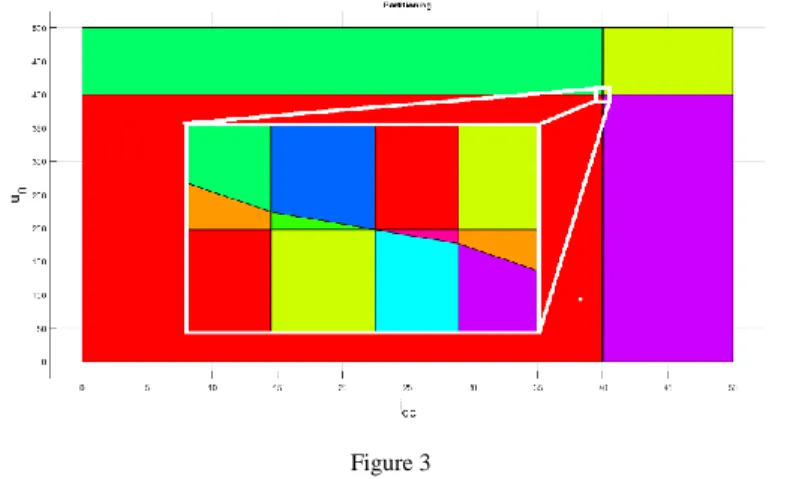
The state space partition resulting from this problem has 13 critical regions, which can be observed in Fig. 3.
Figure 3 State space partitioning
From the basis of the discretized model (9), the given constraints, and horizon (19) the cost function (11) is established via the MPT toolbox [30] and used in the generated controller for the EMPC design [29], [31]. The controller is created as a compliable S-function in the Matlab/Simulink environment and its place in the control structure can be observed in Fig. 4 as the EMPC controller.
The output of the MPC controller is the control variable obtained via solving (12) 𝑢𝑀𝑃𝐶 = (𝛿𝑑𝑢𝑐𝑑+ 𝛿𝑞𝑢𝑐𝑞), from which the current reference can be calculated using (19). The quadrature component 𝑢𝑐𝑞 is zero in the synchronous frame of the filter capacitor voltage.
𝑖𝑟𝑀𝑃𝐶𝑑 =𝑢𝑢𝑀𝑃𝐶
𝑐𝑑 ∙ 𝑖𝑑𝑐 (20)
Figure 4
The control structure of the CSR, with MPC controller on the DC side
3.2 Active AC-Side Damping
The CSR requires a voltage supply on the AC side. Taking into consideration the inductive character of the mains, the presence of a three-phase capacitor tank at the input of the CSR is a must. The most convenient is to use three-phase LC filtering with inductors on the lines and star connected capacitors resembling those in Fig. 1, although the resonance phenomena between these components can still cause difficult problems. The simplest way to dampen the resonance on the AC side LC filter is to add a damping resistor across the capacitor [23]. Because these resistors result in high losses, active damping methods have been proposed, which emulate damping resistors by control. This makes the CSR bridge produce an additional high frequency current, equivalent to the presence of virtual damping resistors connected in parallel with the AC capacitors. The resonance of the AC side LC filter produces harmonics in the capacitor voltage with frequency close to 𝜔𝑎𝑐=√𝐿1
𝑎𝑐𝐶𝑎𝑐, which appears as 𝜔𝑎𝑐− 𝜔𝑠 component in 𝑢𝑐𝑑, where 𝜔𝑠= 2𝜋𝑓.
The fundamental component of the capacitor voltage represents a DC component in the synchronous reference frame. Therefore, a high-pass filter (HPF) is applied to filter out this DC component, with the transfer function:
𝐻𝑃𝐹(𝑠) = 𝑠
𝑠 + 0.1 ∗ (𝜔𝑎𝑐− 𝜔𝑠) . (21)
A virtual damping resistance 𝑅𝐻 has been defined for calculation of the damping current component 𝑖𝐻𝑃𝐹 from the HF component of the capacitor voltage.
4 Space Vector Modulation Strategy
The chosen modulation strategy is developed in the “αβ” stationary reference frame. The structure requires simultaneous conduction of the upper and lower transistors of the bridge, since the current of the 𝐿𝑑𝑐choke must not be interrupted.
Additionally, the switching devices are considered as ideal.
Figure 5
The fundamental input current vectors corresponding to the active switching states of the CSR According to this, one of the upper and one of the lower switches must be closed at all times. This allows nine states, six of which are active. There are three “zero”
vectors, corresponding to the switching states, when both devices of one of the bridge legs are in conduction, shown in Table 1.
Table 1
Switching states of the rectifier and the corresponding space phasors Name Switching State Phase currents Vector representation
1 2 3 4 5 6 ia ib ic
𝑖1
⃗⃗ 1 0 0 0 0 1 idc 0 -idc (2𝑖𝑑𝑐𝑒(𝑗𝜋6)) √3⁄ 𝑖2
⃗⃗ 0 0 1 0 0 1 0 idc -idc (2𝑖𝑑𝑐𝑒(𝑗𝜋2)) √3⁄ 𝑖3
⃗⃗ 0 1 1 0 0 0 -idc idc 0 (2𝑖𝑑𝑐𝑒(𝑗5𝜋6)) √3⁄ 𝑖4
⃗⃗ 0 1 0 0 1 0 -idc 0 idc (2𝑖𝑑𝑐𝑒(𝑗7𝜋6)) √3⁄ 𝑖5
⃗⃗ 0 0 0 1 1 0 0 -idc idc (2𝑖𝑑𝑐𝑒(𝑗3𝜋2)) √3⁄ 𝑖6
⃗⃗ 1 0 0 1 0 0 idc -idc 0 (2𝑖𝑑𝑐𝑒(𝑗11𝜋6 )) √3⁄ 𝑖7
⃗⃗ 1 1 0 0 0 0 0 0 0 0
𝑖8
⃗⃗ 0 0 1 1 0 0 0 0 0 0
𝑖9
⃗⃗ 0 0 0 0 1 1 0 0 0 0
The neighboring space phasors can be formulated as:
𝑖𝑛
⃗⃗⃗ = 2
√3𝑖𝑑𝑐𝑒𝑥𝑝𝑗 (𝑛𝜋 3 −𝜋
6) 𝑖𝑛+1
⃗⃗⃗⃗⃗⃗⃗ = 2
√3𝑖𝑑𝑐𝑒𝑥𝑝𝑗 (𝑛𝜋 3 +𝜋
6) 𝑛 = 1,2, … 6
(22)
The reference current vector is sampled with fixed sampling period Ts. The sampled value of 𝑖⃗⃗⃗⃗⃗⃗⃗ is synthesized as the time average of two neighbouring 𝑟𝑒𝑓
space phasors adjacent to the reference current:
𝑇𝑛𝑖⃗⃗⃗ + 𝑇𝑛 𝑛+1𝑖⃗⃗⃗⃗⃗⃗⃗ = 𝑇𝑛+1 𝑠𝑖⃗⃗⃗⃗⃗⃗⃗ . 𝑟𝑒𝑓 (23) 𝑇𝑛 and 𝑇𝑛+1 represent the individual durations of the switching states corresponding to the neighboring vectors. For example, in case of a current reference vector situated in the first sector, T1, T2 and T0 can be calculated using (24).
𝑇1= 𝑇𝑠𝑖𝑟𝑒𝑓𝛼 𝑖𝑑𝑐 𝑇2= 𝑇𝑠√3
2 1
𝑖𝑑𝑐(𝑖𝑟𝑒𝑓𝛽− 1
√3𝑖𝑟𝑒𝑓𝛼) 𝑇0= 𝑇𝑠− 𝑇𝑛− 𝑇𝑛−1= 𝑇7,8,9
(24)
Figure 6
Synthesis of 𝑖⃗⃗⃗⃗⃗⃗ by 𝑖𝑟𝑒𝑓 ⃗⃗ , 𝑖1 ⃗⃗ , and 𝑖2 ⃗⃗ 0
The complex plane is naturally divided by the fundamental space vectors into six areas, named “sectors”.
𝜋
6+(𝑛 − 1)𝜋
3 ≤ 𝜃𝑛≤𝜋 6+𝑛𝜋
3 𝑛 = 1,2, … 6
(25)
The non-zero space vectors are selected based on the phase angle 𝜃 between 𝑖⃗⃗⃗⃗⃗⃗⃗ 𝑟𝑒𝑓 and the real axis. Table 2 presents an example of switching pattern in case of a current reference vector situated in Sector I.
Table 2
Representation of switching sequences for SECTOR I 𝑖1
⃗⃗ 𝑖⃗⃗ 2 𝑖⃗⃗ 9 𝑖⃗⃗ 9 𝑖⃗⃗ 2 𝑖⃗⃗ 1
S1
S2
S3
S4
S5
S6
Ts Ts
The switching scheme represented in Table 1 is aimed at reducing the number of commutations in a switching cycle, resulting in the reduction of the switching losses [32]. Additionally, the constraint (26) resulting from the available magnitudes of the current vectors, is applied to the current reference.
0 ≤ |𝑖𝑟𝑒𝑓| ≤ √6𝑖𝑑𝑐
𝑐𝑜𝑠(𝜃) + √3𝑠𝑖𝑛(𝜃)
(26)
5 Performance Evaluation
From the continuous AC (5), and DC (6) model equations described in Ch. 2, the controller is formulated form discretised system (9), and it is described via the cost function and control problem of (11), and (12) in Ch. 3. The evaluated model and control structure are shown on Fig. 4. In the following section said EMPC’s computational requirements are evaluated, and the Matlab/Simulink simulation results are compared to a classic state feedback controller’s dynamic performance.
5.1 Computational Effort
The binary search tree generated for the control problem presented in Fig. 7, and described in Ch. 3. The depth of the search tree is 5 and it has a total number of 29 nodes. It is utilized with the MPT toolbox [30], [31], [33] and it can be used for the computationally optimal real-time implementation of the proposed algorithm on low-cost hardware.
Figure 7
Binary search tree of the controller for a horizon of N=4. The leaf nodes are depicted with filled squares. The depth of the tree is 5.
The search for an active critical region starts from the first level and represents the evaluation in each adjacent node of an inequality of the form: 𝑥 ≤ 𝐾. Thus, in this case a maximum number of 4 inequalities have to be evaluated to reach the active critical region. Implementing the presented algorithm is straightforward on a DSP processor, for instance from the dsPIC33 family by Microchip. Using the mac (multiply and accumulate) instruction the inequality is evaluated for each node using 4 instructions, thus in 80 ns on a 50 MIPS processor (Fig. 8). The active critical region can be reached in a maximum of 400 ns. Compared to the typical sample rate of 10us in the case of a CSR, the real-time implementation on a DSP processor is possible.
h11
h12
h21
h22
hn2
H 0 k1
0
k2
kn
K x1
x2
x
6 5
6 10 5 8 6 5
6 10
5 8 10 8
1 2 12 1 11
*
, , , , ,
* , ,
w w mac
w w w w A w w mac
w w mov
w w mov
x w
H w
k x h x h
Figure 8
Data organization in the data memory of a single core DSP and the evaluation of a 2-dimensional inequality
5.2 Horizon Performance
With the cost function (11) employed using (18), changing the length of the horizon (N) affects the system’s complexity illustrated by the partition in the state space shown in Fig. 3, and Fig. 11 presents the step response of the controlled system for different lengths of the horizon. It shows, that the response is not affected by the increase of the horizon above N=2, supporting the choice of this value for Matlab Simulink implementation.
Figure 9
Step response of the system as a function of the horizon length (N)
5.3 Simulation Results
The simulation results are produced with Matlab/Simulik. The discrete model’s (9) simulation frequency was 𝑓𝑠= 106𝐻𝑧, with the model parameters represented in Table 3, and with the control structure shown on Fig. 4. The EMPC performance is shown in Fig. 10 and Fig. 11.
Figure 10
Three-phase voltage and current intake of the CSR with EMPC
Figure 11
Resulting current and voltage trajectories of the CSR with (EMPC)
More details about the Matlab simulation are presented in [34].
5.4 Comparison with a State Feedback Control
On the DC side, not only the output voltage 𝑢0 but also the inductor current 𝑖𝑑𝑐
needs to be controlled. Described in [28], a state feedback control with optimal parameters can be used as a reference based on the model properties listed in Table 3, with output voltage 𝑢0 and DC bus current 𝑖𝑑𝑐 chosen as the state
variables. Since 𝑢0 is a DC quantity in steady state, an integrator signal is introduced to diminish the steady-state error. The structure of the controller is represented in Fig. 12.
Figure 12
Simple DC side state feedback control structure The tuning constants applied and calculated according to [24] are:
𝑘1 =1.5𝑈𝜔𝑛3
𝑛𝜔𝑑𝑐2 , 𝑘2 =1.9𝜔1.5𝑈𝑛𝐿𝑑𝑐
𝑛 , 𝑘3 =1.5𝑈2.2𝜔𝑛2
𝑛(𝜔𝑑𝑐2 −1), (26)
where 𝜔𝑛= 1.1, 𝜔𝑎𝑐=√𝐿1
𝑎𝑐𝐶𝑎𝑐 , and 𝜔𝑑𝑐 =√𝐿1
𝑑𝑐𝐶𝑑𝑐.
The state feedback controllers block on the diagram is taking the controller’s place, shown on Fig. 2. The independent outputs are the high pass filter’s output 𝑖𝑟𝐻𝐹(𝑑) and the controller’s output 𝑖𝑟𝑐𝑜𝑛𝑡𝑟𝑜𝑙(𝑑). The sum of the independent current values is converted to Clarke frame to be able to govern the switching states of the IGBT’s. This can be done because 𝑖𝑟𝐻𝐹(𝑑) has only high frequency components and 𝑖𝑟𝑐𝑜𝑛𝑡𝑟𝑜𝑙(𝑑) has low frequency components due to the differences in LC time constants, as discussed in the second section. Then, the control signal governing the switches is applied in the same manner, described at the start of Section 3. The state feedback control’s performance in comparison with the EMPC is shown in Fig. 13.
Figure 13
Resulting current and voltage trajectories of the CSR with explicit model predictive control (MPC) compared state feedback control (SF), and simple proportional-integral control (PI), where 𝑃 = 0.01,
and 𝐼 = 100, with the respect of constraints described in (19)
Appendix
Table 3
The applied parameters in model and controller design
Parameter Value Description
𝑅 0.3 𝛺 Phase resistance
𝑅𝑙𝑜𝑎𝑑 10 𝛺 Load resistance
𝐿𝑎𝑐 1 𝑚𝐻 AC-side filter inductance
𝐿𝑑𝑐 30 𝑚𝐻 Choke inductance
𝐶𝑎𝑐 30 𝜇𝐹 AC-side filter capacitance
𝐶𝑑𝑐 400 𝜇𝐹 DC-side capacitance
𝑓𝑠 10−6𝐻𝑧 Simulation frequency
𝑓 50 𝐻𝑧 Network frequency
𝑓𝑝𝑤𝑚 20 𝑘𝐻𝑧 Modulation frequency
𝑈𝑛 400 V Network line voltage
𝑅𝑤 𝑰2 State weighting matrix
𝑄𝑤 10−6𝑰2 Input weighting matrix
N 2 Control horizon
ωn 1.1 undamped oscillation frequency
Conclusions
The constrained, model-based optimal control of a current source rectifier has been presented in this paper. The dynamic model of a three-phase current source rectifier has been developed in Park frame. The proposed model has been examined from the design and implementation points of view with the purpose of explicit model-based predictive control. It proved to be the case that the regular set of differential equations of the CSR appears to be too complex, and contains non- linearity for such a design approach. To address this issue the usage of separated AC and DC equation sets was suggested to avoid linearization and complexity reduction. This solution eliminates bilinearity and enables the application of linear control design techniques. Current-based SVPWM of the three-phase converter has been used with an emphasis on the reduction of switching losses. Throughout the article the explicit model predictive control method is described and the method's effectiveness compared to conventional state feedback control is show.
The implementation and simulation experiments have been performed in Matlab/Simulink environment. Moreover, the proper implementation of the system in a modern DSP chip will result in real-time operation.
Acknowledgement
Attila Fodor acknowledges the financial support of Széchenyi 2020 under the EFOP-3.6.1-16-2016-00015. Attila Magyar was supported by the János Bolyai Research Scholarship of the Hungarian Academy of Sciences.
References
[1] I. Vajda. Y. N. Dementyev, K. N. Negodin, N. V. Kojain, L. S. Udut, Irina.
А. Chesnokova: Limiting Static and Dynamic Characteristics of an Induction Motor under Frequency Vector Control, Acta Polytechnica Hungarica, Vol. 14, No. 6, 2017
[2] B. Ghalem, B. Azeddine: Six-Phase Matrix Converter Fed Double Star Induction Motor, Acta Polytechnica Hungarica, Vol. 7, No. 3, 2010
[3] S. Gupta, R. K. Tripathi: Two-Area Power System Stability Improvement using a Robust Controller-based CSC-STATCOM, Acta Polytechnica Hungarica, Vol. 11, No. 7, 2014
[4] Y. Li, P. Li, Y. Chen, D. Zhang: Single-stage three-phase current-source rectifier for photovoltaic gridconnected system, Conference of Power Electronics and Applications (EPE'14-ECCE Europe), Finland, 2014 [5] B. Exposto, R. Rodrigues, J. G. Pinto, V. Monteiro, D. Pedrosa, J. L.
Afonso: Predictive Control of a Current-Source Rectifier for Solar Photovoltaic Grid Interface, Compatibility and Power Electronics (CPE) Conference, Portugal, 2015
[6] M. Chebre, A. Meroufel, Y. Bendaha: Speed Control of Induction Motor Using Genetic Algorithm-based PI Controller, Acta Polytechnica Hungarica Vol. 8, No. 6, 2011
[7] R. Salloum: Robust PID Controller Design for a Real Electromechanical Actuator, Acta Polytechnica Hungarica, Vol. 11, No. 5, 2014
[8] L. Neukirchner, P. Görbe, A. Magyar: Voltage unbalance reduction in the domestic distribution area using asymmetric inverters, Journal of Cleaner Production Vol. 142, Part 4, 20 January 2017, pp. 1710-1720
[9] F. Tahri, A. Tahri, A. Allali and S. Flazi: The Digital Self-Tuning Control of Step a Down DC-DC Converter, Acta Polytechnica Hungarica, Vol. 9, No. 6, 2012
[10] H. Gao, D. Xu, B. Wu, N. R. Zargari: Model Predictive Control for Five- level Current Source Converter with DC Current Balancing Capability, Industrial Electronics Society , IECON 2017 - 43rd Annual Conference of the IEEE, China, 2017
[11] Y. Han, L. Xu, M. M. Khan, C. Chen: Control Strategies, Robustness Analysis, Digital Simulation and Practical Implementation for a Hybrid APF with a Resonant Ac-link, Acta Polytechnica Hungarica, Vol. 7, No. 5, 2010
[12] T. Venkatraman, S. Periasamy: Multilevel Rectifier Topology with Modified Pulse Width Modulation and Reduced Switch Count, Acta Polytechnica Hungarica, Vol. 15, No. 2, 2018
[13] H. Feroura, F. Krim, B. Tabli, A. Laib: Finite-Set Model Predictive Voltage Control for Islanded Three Phase Current Source Rectifier, Conference of Electrical Engineering - Boumerdes (ICEE-B) Algeria, 2017
[14] Z. Yan, X. Xu, Z. Yang, X. Wu: Study of Effective Vector Synthesis Sequence for Three-Phase Current Rectifier, Fifth International Conference on Instrumentation and Measurement, Computer, Communication and Control (IMCCC) IEEE, 2015, pp. 1065-1070
[15] A. Ürmös, Z. Farkas, M. Farkas, T. Sándor, L. T. Kóczy, Á. Nemecsics:
Application of self-organizing maps for technological support of droplet epitaxy, Acta Polytechnica Hungarica, Vol. 14, No. 4, 2017, pp. 207-224 [16] A. Chatterjee, R. Chatterjee, F. Matsuno, T. Endo: Augmented stable fuzzy
control for flexible robotic arm using LMI approach and neuro-fuzzy state space modeling, IEEE Transactions on Industrial Electronics, Vol. 55, No.
3, 2008, pp. 1256-1270
[17] T. Haidegger, L. Kovács, R. Precup, B. Benyó, Z. Benyó, S. Preitl:
Simulation and control for telerobots in space medicine, Acta Astronautica, Vol. 181, No. 1, 2012, pp. 390-402
[18] S. Vrkalovic, E. Lunca, I. Borlea: Model-free sliding mode and fuzzy controllers for reverse osmosis desalination plants, International Journal of Artificial Intelligence, Vol. 16, No. 2, 2018, pp. 208-222
[19] C. B. Regaya, A. Zaafouri, A. Chaari: A New Sliding Mode Speed Observer of Electric Motor Drive Based on Fuzzy-Logic, Acta Polytechnica Hungarica, Vol. 11, No. 3, 2014
[20] K. Széll, P. Korondi: Mathematical Basis of Sliding Mode Control of an Uninterruptible Power Supply, Acta Polytechnica Hungarica, Vol. 11, No.
3, 2014
[21] A. Kelemen, N. Kutasi, M. Imecs, I. I.I ncze: Constrained Optimal Direct Power Control of Voltage-Source PWM Rectifiers, International Conference on Intelligent Engineering Systems (INES) IEEE International Conference, Las Palmas of Gran Canaria, Spain, 2010
[22] A. Tahri, H. M. Boulouiha, A. Allali and T. Fatima: Model Predictive Controller-based, Single Phase Pulse Width Modulation (PWM) Rectifier for UPS Systems, Acta Polytechnica Hungarica, Vol. 10, No. 4, 2013 [23] M. Rivera, S. Kouro, J. Rodriguez, B. Wu, V. Yaramasu, J. Espinoza and P.
Melin: Predictive Current Control in a Current Source Rectifier Operating with Low Switching Frequency, 4th International Conference on Power Engineering, Energy and Electric Drives, Turkey, 2013
[24] A. Godlewska, A. Sikorski: Predictive control of current source rectifier, Selected Problems of Electrical Engineering and Electronics (WZEE), IEEE, 2015, pp. 1-6
[25] N. Muthukumar, S. Srinivasan, K. Ramkumar, K. Kannan, V. E. Balas:
Adaptive Model Predictive Controller for Web Transport Systems, Acta Polytechnica Hungarica, Vol. 13, No. 3, 2016
[26] N. Kutasi, A. Kelemen, M. Imecs: Constrained Optimal Control Of Three- Phase AC-DC Boost Converters, Automation Quality and Testing Robotics (AQTR) IEEE International Conference, Cluj-Napoca, Romania, 2010 [27] S. F. Ahmed, Ch. F. Azim, H. Desa, A. T. Hussain: Model Predictive
Controller-based, Single Phase Pulse Width Modulation (PWM) Rectifier for UPS Systems, Acta Polytechnica Hungarica, Vol. 11, No. 6, 2014 [28] Y. Zhang, Y. Yi, P. Dong, F. Liu, Yong Kang: Simplified Model and
Control Strategy of Three-Phase PWM Current Source Rectifiers for DC Voltage Power Supply Applications, IEEE Journal of emerging and selected topics in power electronics, Vol. 3, No. 4, december 2015
[29] A. Bemporad, M. Morari, V. Dua, Efstratios N. Pistikopoulos: The explicit linear quadratic regulator for constrained systems. Automatica Vol. 38, 2002, pp. 3-20
[30] M. Herceg, M. Kvasnica, C. N. Jones, M. Morari: Multi-Parametric Toolbox 3.0, Proceedings of the European Control Conference, Zürich, Switzerland, 2013, pp. 502-510
[31] N. Kutasi, A. Kelemen, Sz. Matyasi, M. Imecs: Hardware implementation of explicit mode-predictive control of three phase PWM rectifiers, ICCC2010 Eger, Hungary, 2010, pp. 133-136
[32] L. Moussaoui, A. Moussi: An open loop space vector PWM control for CSR-fed field oriented induction motor drive with improved performances and reduced pulsating torque, Proceedings of the 6th WSEAS international conference on Automation & information, March 2005, Part 4. pp. 329-335 [33] M. Kvasnica, I. Rauová and M. Fikar: Automatic code generation for real- time implementation of Model Predictive Control, 2010 IEEE International Symposium on Computer-Aided Control System Design, Yokohama, 2010, pp. 993-998
[34] L. Neukirchner: Constrained Predictive Control of Three-Phase BuckRectifiers Simulation details, http://virt.uni- pannon.hu/ver/index.php/en/projects/30-empc-csr, 2019