Drive Control

(1)

Drive Control

BMEVIVEM175

Schmidt, István

Veszprémi, Károly

(2)

Drive Control

írta Schmidt, István és Veszprémi, Károly Publication date 2012

(3)

Ajánlás

The authors acknowledge the review work and advices of Prof. Mátyás Hunyár, the typing of Mrs. Écsi Antalné, the drawings of Miss Ilona Wibling.

(4)

Tartalom

Preface ... iii

1. Introduction ... 1

2. Commutator DC machines ... 3

1. Separately excited DC machine ... 3

2. Converter-fed DC drives ... 5

2.1. Line commutated converter-fed DC drives ... 5

2.2. DC Chopper-fed DC drives ... 10

2.3. Implementations of the current controllers ... 12

2.4. Operation extended by field-weakening range ... 16

3. Park-vector equations of the three-phase synchronous and induction machines ... 18

4. Permanent magnet sinusoidal field synchronous machine drives ... 22

1. Operation modes, operation ranges and limits ... 23

2. Field-oriented current vector control ... 25

2.1. Implementation methods ... 25

2.2. Three-phase two-level PWM voltage source inverter ... 26

2.3. Current vector controls ... 28

2.3.1. PWM modulator based current vector controls ... 29

2.3.2. 4.2.3.2 Hysteresis current vector controls ... 33

5. Frequency converter-fed squirrel-cage rotor induction machine drives ... 36

1. Field-oriented control methods ... 36

2. Steady-state sinusoidal field-oriented operation ... 39

3. Implementation methods of the field-oriented operation ... 41

3.1. Field-oriented current vector control ... 41

3.2. Machine models ... 45

4. Direct torque control ... 47

6. Double-fed induction machine drives by VSI ... 52

1. Field-oriented current vector control ... 53

7. Line-side converter of the VSI-fed drives ... 59

1. VSI type line-side converter ... 59

1.1. Line-oriented current vector control of the line-side converter ... 60

8. Current source inverter-fed short-circuited rotor induction machine drives ... 64

1. CSI-fed drives with thyristors ... 64

1.1. Filed-oriented current vector control ... 65

2. Pulse width modulated CSI-fed drives ... 68

9. Converter-fed synchronous motor drive ... 70

10. Switched reluctance motor drive ... 76

11. Speed and position control ... 79

1. Speed control ... 79

2. Position control ... 82

12. Applications ... 87

1. Flywheel energy storage drive ... 87

2. Electrical drives of vehicles ... 91

2.1. Locomotive ... 91

2.2. Trolleybus ... 93

3. Wind turbine generators ... 94

4. Starting of a gas turbine-synchronous generator system ... 98

5. Calculation example ... 100

A. Notations different from international ... 101

Irodalomjegyzék ... 103

(5)

Preface

The electronic lecture notes entitled Drive Control is prepared for the MSc. students of the Budapest University of Technology and Economics, Faculty of Electrical Engineering and Informatics, Specialization of Electrical Machines and Drives. The lecture notes deals with the theoretical and practical investigation of the modern drive-specific and task-specific control methods of the semiconductor electrical drives, containing power electronics and electric motors.

The topic assumes the basic knowledge of the electric machines, power electronics and control theory. Besides, for the investigation of the three-phase semiconductor controlled drives, the knowledge of the Park-vector (space-vector) representation methods is definitely necessary. Those students, graduating at our BSc. courses in Electric Power Engineering specialization have these knowledges.

The figures of this lecture notes have been available for the students for many years as paper copy study material.

Besides the study purpose, this lecture notes can be well utilized by drive designers or specialists applying electric drives.

The content can be extended by the help of references at the end.

Budapest, 2011.

Dr.Schmidt István professor emeritus

Dr.Veszprémi Károly professor

(6)

(7)

1. fejezet - Introduction

In the Drive Control subject motion controls implemented by electric drives are investigated. One-shaft equivalent (referred) model of the system can be derived in mechanically rigid and knocking-free drive chain.

The referring can be done to the shaft of the electric motor or the mechanical load. Fig.1.1. shows the one-shaft model of a rotating system referred to the motor shaft.

Fig.1.1. One-shaft model on the motor shaft. a. Model, b. Positive directions, c. Operation quadrants.

In the figure: m is the motor torque, mt is the load torque, θm is the motor inertia, θt is the inertia of the load, w is the angular speed of the motor shaft, α is its rotation angle. Assuming constant resultant inertia (θ=θm+θt), the motion equation is:

(1.1.a,b)

Where md is dynamic (accelerating) torque. Eq. (1.1.a) is the equivalent expression of Newton‟s II. law for rotation. The motion parameters: the dw/dt angular acceleration, the w angular speed and the α rotation angle can be controlled by the motor torque m. The mt load torque can be considered as disturbance.

A modern controlled drive contains an electric motor, a power electronic circuit and a drive controller (see Fig.

1.2).

Fig.1.2. Block-scheme of a controlled electric drive.

The drive controller usually operates in subordinated structure. Assuming position control, Fig.1.3. shows the block-scheme of the drive control. The aim is tracking the αa position reference.

Fig. 1.3. Subordinated (cascaded) structure of the position control.

According to the subordinated structure, the position controller provides the wa speed reference, the speed controller provides the ma torque reference, the torque controller provides the ia current reference. The current controller controls the power electronics by the v control signal. α, w, m and i are the feedback signals of the angle, speed, torque and current respectively. The current control is drive-specific, the position control is drive- independent (task-specific). The speed control is usually drive-independent, but there are drive-specific versions (sensorless). There is not explicit torque control, since it can be deduced to current control. There is always a current control. Its aim is to control the torque and perhaps the flux, furthermore to perform overload (overcurrent) protection.

The controlled electrical drives can be found in every modern equipment, in the developed country they consume approx. the half of the produced electric power.

(8)

Introduction

First the drive-specific current and torque controls are investigated for DC, synchronous, induction and reluctance machines. Then the task-specific speed and position controls are discussed and some practical applications are presented.

Among the synchronous and induction motor drives only the control of the modern, widely applied DC link frequency converter-fed drives are investigated.

(9)

2. fejezet - Commutator DC machines

First the DC machines, then the supplying power electronics and finally the current controllers are discussed.

1. Separately excited DC machine

The separately excited, permanent magnet and series excited DC machines are applied in practice. Separately excited, compensated DC machine is assumed in the following. Its equivalent circuit in one-shaft model is shown in Fig.2.1.

Fig.2.1. Equivalent circuit

Fig.2.2. Mechanical characteristics.

The input signals of the motor are the u terminal voltage and the ϕ=f(ig) flux, its output signals are the I armature current, the m toque, the w speed and the α angle, disturbance signal is the mt load troque. Assuming ϕ=const.

and θ=const., the drive equations are summarized in (2.1-2.5):

u(t)=Ri(t)+L·di(t)/dt+ub(t), u(s)=Ri(s)+Lsi(s)+ub(s). (2.1.a,b)

ub(t)=kϕw(t), ub(s)=kϕw(s). (2.2.a,b)

m(t)-mt(t)=θ·dw(t)/dt, m(s)-mt(s)=θsw(s). (2.3.a,b)

m(t)=kϕi(t), m(s)=kϕi(s). (2.4.a,b)

w(t)=dα(t)/dt, w(s)=sα(s). (2.5.a,b)

(10)

Commutator DC machines

pm=ubi, since the brush, core, friction and ventilation losses are neglected at the rotor. In steady-state: di/dt=0 and dw/dt=0. Considering these, from the expressions of column “a” the W(M) mechanical characteristic of the drive can be expressed:

(2.6.a,b)

Accordingly, for a given M torque the w speed can be modified by U, ϕ and R (the last one is lossy). In controlled drives mainly the U terminal voltage (the W0=U/kϕ no-load speed) is modified. By the ϕ flux (field- weakening) the speed range can be extended. Assuming 4/4 quadrant operation Fig.1.2. presents the linear W(M) mechanical characteristics (U=const. and ϕ=const.) for the normal (ϕ=ϕn, -Un≤U≤Un) and for the field- weakening (U=Un, or U=-Un, ϕ<ϕn, ϕ=ϕn│W0n/W0│≈ϕn│Wn/W│) ranges. The long-time loadability limit corresponding to I=±In nominal current is also shown. Eg. in the W>0 and M>0 quadrant at the normal range maximum M=Mn=kϕnIn nominal torque is allowed, while in field-weakening maximum Pm=MW=UbI=MnWn=Pn

nominal power is allowed.

Using the column “b” in (2.1-2.5):

(2.7.a,b)

the block-diagram of the constant flux DC machine can be drawn (Fig.2.3., Tv=L/R is the electric time constant of the armature circuit).

Fig.2.3. Block-diagram for ϕ=const.

For linear system the superposition can be applied, so e.g. the w speed can be calculated as

(2.8)

The Ywu and Ywmt transfer functions can be derived from the block-diagram:

(2.9)

(2.10)

Here: Tm=θR/(kϕ)²=-θ·dW/dM is the electromechanical time constant for mt=const, is the equivalent time constant, is the damping factor. If ξ>1 (i.e. Tm>4Tv), then aperiodic, if ξ<1 (i.e. Tm<4Tv), then oscillating speed tracking is got for a step change in terminal voltage or load torque. With s=0 (t=∞) the transfer factors are the same as the factors got from (2.6.a) for steady-state. For the inner part of Fig.2.3. the voltage-dimension block diagram (Fig.2.4) or the per-unit dimensionless block diagram (Fig.2.5) are frequently used. In the latest, the quantities are dimensionless, they are related to the nominal values: u‟=u/Un,

(11)

i‟=i/In, ϕ‟=ϕ/ϕn, m=m/Mn, w‟=w/W0n, R‟=RIn/Un, Tin=θW0n/Mn=θW0nWn/Pn is the nominal starting time, Tm/Tin=(W0n-Wn)/W0n=R‟. For the motors Tv and Tm are few tens ms, Tin is few hundreds ms.

Fig.2.4. Voltage dimension block-diagram.

Fig.2.5. Per-unit block-diagram.

2. Converter-fed DC drives

The DC machine is fed by the converter ÁI (Fig.2.6). The converter can be line-commutated AC/DC converter or DC/DC chopper. In both cases the uk mean value of the pulsating u terminal voltage of the converter (and so the w=wk speed of the drive) can be controlled continuously. The expression (2.6) is valid here also, but the Uk, Ik, Mk mean values must be substituted. The speed pulsation can be neglected (w≈wk) because of the

integration (1.1.a). A filter choke with LF and RF parameters is inserted frequently between the converter and the motor to reduce the pulsation of the I current and m torque. So in (2.6.a) R+RF must be used instead of R.

Fig.2.6. Converter-fed DC drive.

2.1. Line commutated converter-fed DC drives

For AC/DC line commutated converter in an industrial drive most commonly three-phase, six-pulse symmetrically controlled thyristor bridge is applied. In this case the pulsation frequency of the u voltage, i current and m torque is f0=6fh=6·50 Hz=300 Hz, the pulse time is . The equivalent circuit is in Fig.2.7. and the output characteristic Uk(Ik) is in Fig.2.8.

(12)

Fig.2.7. Three-phase thyristor bridge DC drive.

Fig.2.8. The Uk(Ik) characteristic of the three-phase thyristor bridge.

The transformer (or commutation coil) is represented by its equivalent circuit in Fig.2.7. The Ikr=f(α) critical current curve is the border of the continuous and discontinuous conduction modes in Fig.2.8. At Ik>Ikr current (e.g. in point 1) the conduction is continuous, at Ik<Ikr (eg. in point 2) it is discontinuous. In quadrant I. the converter is in rectifying mode, in quadrant IV. it is in inverter mode. Using R=RF=0 approximation, Uk=Ub and so Fig.2.8. shows the W(M) mechanical characteristic (at ϕ=const.) approximately. As it can be seen, the thyristor bridge drive is capable of 2/4 quadrant operation (quadrants I. and IV. in Fig.1.1.c.).

At continuous conduction the Uk(Ik) characteristic is linear:

(2.11.a,b,c)

Where: is the mean value of the maximal continuous operation voltage, Rf=(3/π)ωhLt is a fictive resistance caused by the overlap (Utm is the peak value of the phase voltage, ωh=2πfh is the angular frequency of the lines).

For transients in continuous conduction mode (Fig.2.9.a) the approximating equivalent circuit in Fig.2.9.b. can be drawn for the important mean values.

Fig.2.9. Transient operation in continuous mode. a. Time function of the current/torque instantaneous and mean value. b. Equivalent circuit.

Accordingly, a similar armature voltage equation with mean values can be used as in (2.1.a) for the transient process:

(2.12)

(13)

(2.13.a,b)

For α input value Eq. (2.12) is nonlinear caused by cosα, so small deviations should be considered and the equation must be linearized. Assuming constant phase voltage amplitude (so Ukm=const.) uko depends only on α:

(2.14)

Using Laplace transformation and rearranging:

(2.15.a,b)

Here: Tve=Le/Re. For the w speed and ub induced voltage the k index marking mean value can be omitted, since these quantities can not follow the torque pulsation with fo=6fh=300Hz frequency (w=wk, ub=ubk). Using (2.15) and Fig. 2.3. the block diagram valid for continuous conduction mode can be drawn (Fig.2.10.).

Fig.2.10. Block diagram of the thyristor bridge DC drive for continuous conduction mode.

The dead time should be considered by the factor , since Δuk0 can be modified only after the firing. The average dead time is . As can be seen from the block diagram, the transfer function of the GV firing controller is also necessary. uv is the input signal of the firing control, at analogue implementation it is a control voltage. It is usual to make nonlinear firing control, to get cosα proportional to uv. In this way the nonlinearities of GV and ÁIF compensate each other, i.e. the relation between uv and uko becomes linear.

For discontinuous conduction the Uk(Ik) characteristic is nonlinear (see Fig.2.8.). In this case ik can step-change during transients, since the current i starts from zero value at the beginning of every pulse, and becomes zero at the end of the pulse. This is demonstrated in Fig.2.11. for Δα decrease.

Fig.2.11. The time function of the current instantaneous and mean value for discontinuous conduction.

Using mean values averaged to T0 pulse period, according to Fig.2.6. and Fig.2.8. the following voltage equation can be written:

(2.16)

There are no inductances in the expression, since ik can step change. It must be linearized, since according to Fig.2.8. uk is nonlinearly depends on α and ik:

(2.17)

Linearizing (2.16), using Laplace transform and rearranging:

(14)

(2.18.a,b,c)

Using this expression, the block diagram for discontinuous conduction can be drawn.

Fig.2.12. Block diagram of the thyristor bridge DC drive for discontinuous conduction mode.

Resz (2.18.b) is much larger than Re (2.13.a). It comes from the fact that both RÁI, and RÁISZ are proportional to the gradient of the static (steady-state) Uk(Ik) characteristic at the given point (e.g. points 1 and 2 in Fig.2.8.) and RÁISZ>>RÁI.

Comparing Fig.2.10. and Fig.2.12. it is clear, that there is a significant difference between the block diagrams of the continuous and discontinuous conduction. Consequently, different type current controllers are necessary in the two operation modes. The Th dead time will be neglected during the investigation of the current control.

The three-phase thyristor bridge drive (Fig.2.7-2.8.) is capable of two quadrant (2/4) operation (quadrant I. and IV. in Fig. 2.2.). The block diagram of the current control loop is given in Fig. 2.13. According to (2.4.a) the current control corresponds to indirect torque control.

Fig.2.13. The block diagram of the current control loop in 2/4 operation.

Both the ia current reference and the i current feedback signal can be only positive. The current control loop implements the torque control (ma≥0 is possible), the current limitation (Ikorl) and the firing angle limitation (0≤α≤αmax=150-160⁰, Uvkorl).

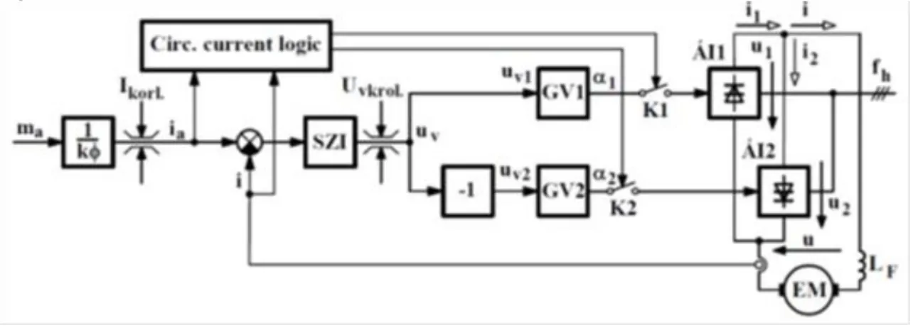
For four-quadrant (4/4) operation two thyristor bridges are necessary, which are practically connected anti- parallely (Fig.2.14.). The ÁI1 converter can conduct i>0, while the converter ÁI2: i<0.

Fig.2.14. Anti-parallel connected 4/4 drive.

(15)

The current control of the two sets converters can be implemented with circulating-current or circulating- currentless control.

Fig.2.15. shows the block diagram of the circulating-currentless control. The circulating-current logic ensures by the K1 and K2 electronic switches, that always only one converter is fired. In this way circulating-current can not develop, so there is no need for any Lk circulating-current limiting chokes. The GV1 firing controller is controlled by uv1=uv, while GV2 by uv2=-uv signal. The later negative sign is necessary to get the same operation for the converters in the reverse rotation but the same operation mode quadrants (I-III. driving, II-IV. braking, Fig. 1.1.c).

Fig.2.15. The current control loop in 4/4 quadrant circulating-currentless operation.

Fig. 2.16.demostrates a transient process, where the ma torque reference is provided by an external speed controller (according to Fig.1.3). A step decrease in point 1 instant is assumed in the na speed reference. For Mt=const. load torque the operation of the drive is transferred from the driving point 1 to the driving point 3, meanwhile the drive is braking. In this case a T0=1-2ms currentless period must be ensured between the reversal of ik armature current for the recovery of the insulation capability of the previously conducting thyristors. The avoidless discontinuous condunctions slow down the reversal of ik current. The overshoot of the ik current in point 2 (thin line) can be avoided, if α2 is set correspondingly to ub=kϕw. In circulating-currentless mode the reversal of the armature current is executed slowly, in more ms.

Fig.2.16. The transient process. a. As a function of time. b. On the w(mk) plane.

Fig.2.17. shows the block diagram of the control with circulating-current. In this case both converters are fired always simultaneously. The basic aim is to provide the same output voltage mean value by both converters (U1=U2). By uk=uko approximation (Fig.2.9.b.):

(2.19.a,b)

(16)

Fig.2.17. The current control loop in 4/4 quadrant circulating-current operation.

Because of the rule for the firing angles of the two converters e.g. from αmax=150ô, αmin=30ô is resulted in. As a result, the utilization of the converters is decreased, since this operation is possible in the cosαmax=- 0,87≤uk0/Ukm≤0,87=cosαmin range. In spite of the equality of U1k and U2k mean values, the u1 and u2 instantaneous values are different, consequently circulating current will flow. This is limited by the Lk chokes. The circulating current results in a faster motor current reversal comparing with the circulating-currentless operation. There are other possible control methods: circulating-current-weak control with α1+α2>180ô and circulating-current regulation. The later needs two current controller: one of them controls to ika, the other to ia+ika (ia is the reference of the motor current, ika is the reference of the circulating current).

All discussed current control (Fig.2.13., 2.15., 2.17.) regulate the mean value of the motor current ik (Fig.2.9., 2.11.) and accordingly the mean value of the motor torque mk=kϕik.

2.2. DC Chopper-fed DC drives

The DC/DC converter can be 1/4, 2/4 and 4/4 quadrant chopper (Fig.2.18.b.) on the Uk(Ik) plane. In this chapter only the 4/4 quadrant version is investigated, since this is applied widely with permanent magnet DC motor in servo and robot drives. The circuit diagram is given in Fig.2.18.a.

Fig.2.18. 4/4 quadrant chopper DC drive. a. Circuit diagram. b. Uk, Ik limit ranges.

The circuit composed by two legs is a three-state converter. For controlling the legs, care must be taken to switch on only one transistor (IGBT) in a leg. If both of them are switched on simultaneously (e.g. T1 and T2), then a short-circuit between the P and N bars is formed. Assuming ideal T1-T4 transistors and D1-D4 diodes the u output voltage can be +Ue, -Ue and 0 value. Applying high frequency switchings between these voltage levels, the mean value of the output voltage can be controlled continuously in the range -Ue≤uk≤Ue. This method is the Pulse Width Modulation (PWM). Unipolar and bipolar operation can be distinguished, the bipolar does not use the u=0 voltage value (Fig.2.19.). The mean value of the voltage in bipolar operation is: uk=(2b-1)Ue, In unipolar operation is uk=±bUe (0≤b=tb/Tu≤1).

(17)

Fig.2.19. Voltage time functions. a,b. Unipolar operation. c. Bipolar operation.

The pulsation frequency of the u voltage is fu=1/Tu, which is more kHz in practice. That is why, to smooth the i armature current no series filter choke is necessary, the L inductance of the armature circuit is enough. With 4/4 quadrant chopper there is no discontinuous conduction, the current with ik=0 mean value is continuous also.

Assuming lossless energy conversion chain, the mean value of the powers are: Pmk=MkW=Pk=UkIk=Pek=UeIek. In motor (driving) mode: Iek>0, in generator (braking) mode: Iek<0.

The aim of the current control is to track the ia=ma/kϕ current reference (determined by the torque demand) with zero error: Δi=ia-i=0. It is not possible with the discrete-states chopper. From the (2.1.a) voltage equation using i=ia-Δi, the derivative of the current error can be expressed:

(2.20.a,b)

The e fictive voltage (using the RΔi=0 approximation) means the continuous terminal voltage corresponding to the errorless reference tracking i=ia. The current controller can select from three voltage levels (+Ue, -Ue, 0) in every instant If the selection is optimal, then i current tracks the ia reference with small error (with small switching frequency), i oscillates around ia.

There are two current control methods applied widely in practice: with PWM modulator and with hysteresis control.

The block diagram of the current control with PWM modulator is presented in Fig.2.20.a. Here SZI is a traditional e.g. PI type current controller, the block PWM is a PWM modulator. The PWM modulator generates the v1-v4 two-level control signals from the uv control signal. The PWM modulator in the chopper plays similar role as the GV firing controller in the line commutated converters. The PWM modulator can operate in push- pull or alternate control mode. The push-pull control results in bipolar operation, the alternate control results in unipolar operation. Commonly true for both of them, that the mean value of the chopper output u voltage (uk) is proportional to the uv control signal. If analogue PWM modulator is used, the Au coefficient in the

(2.21)

expression is the voltage amplification factor of the PWM chopper. The current control with PWM modulator regulates the mean value of the armature current: ik.

Fig.2.20. Current control modes. a. With PWM modulator, b. With hysteresis control.

The block diagram of the hysteresis current control is presented in Fig.2.20.b. Here SZI is a hysteresis current controller, which provides directly the v1-v4 two-level control signals. There is no need for an additional element between the SZI current controller and the Chopper (no PWM modulator), since both are discrete-states

(18)

2.3. Implementations of the current controllers

The voltage dimension block diagram of the PWM modulator based current control of the 4/4 quadrant DC chopper-fed DC drive is given in Fig.2.21. The Motor-Load part corresponds to Fig.2.4., R^* is the Ω dimension transfer factor of the current sensor, Ai=R*/R, Δik=ia-ik is the current error. Let‟s assume first the current transients is so fast that the changing of the speed and the induced voltage can be neglected. The second part of the induced voltage in Ub+ub=kϕW+kϕw is zero. So the feedback from ub can be neglected in the small deviation block diagram of the current control loop (Fig.2.21.).

Fig.2.21. The small deviation block diagram of the current control loop.

The practically applied PI type SZI current controller has the following transfer function:

(2.22)

Selecting properly the Ksz, Tsz parameters, the Tv electrical time constant can be eliminated from the current control loop. So the transfer function of the open current control loop is:

(2.23.a,b,c)

The transfer function of the closed current control loop is a first-order lag element:

(2.24)

Consequently the controlled ik current tracks the ia reference by Ti delay:

(2.25.a)

(2.25.b)

The last equation for the Δik current error (2.25.b) is true if ia=const. Then Δik is changing exponentially:

(2.26)

In practice Ti is given by the user (in servo drives it is around 1ms). Knowing it, the PI type SZI controller can be set in the following way (see (2.23.b,c)):

(19)

(2.27.a,b)

As an example let‟s examine the effect of the current reference step:

(2.28)

The characteristic time functions are presented in Fig. 2.22. In Fig.2.22.a. the current controller operates in linear mode, in Fig.2.22.b. it is limited (saturated) at the beginning.

At linear operation for t>0 the following expressions are valid:

(2.29.a)

(2.29.b)

(2.29.c)

The condition of the linear operation is that the demanded uk (2.29.c) has to fall into the range -Ue≤uk≤+Ue. If ΔIo=Iv-Io greater than ΔI0max=Ti·(Ue-Ub-RI0)/L, then uk(t=+0)>Ue is required for the linear operation. In this case for a while saturated (limited) operation occurs.

Fig.2.22. Tracking a current reference step change. a. Linear operation, b. Saturated (limited) operation.

In the 0<t<t ^*; saturated range Uk=Ue (Fig.2.22.b.). The ik current tends to the Ip=(Ue-Ub)/R steady-state value by exponential function with Tv time constant:

(20)

(2.30)

At t* time instant . In the time interval next to saturation t>t* linear operation occurs, and similarly to (2.29.a) the current time function is:

(2.31)

if at t=t* time instant the integrator of the PI controller sets voltage. This can be ensured by setting the integral part of the uv=uvp+uvI control voltage to uvI=(Ub+Rik)/Au during the saturated operation. As an approximate solution the output of the integrator can be kept on the value which was at the beginning of the saturation (in our example it is uvI=(Ub+Ri0)/Au).

In servo motors because of , neglecting the variation of the ub induced voltage in Fig.2.21. is not allowed. In this case the effect of the ub on the current control loop can be compensated by a feedback (Fig.

2.23.) If the ub part of the terminal voltage uk is set by the compensating feedback, the current controller sees a passive R-L circuit:

(2.32)

Fig.2.23. Applying compensating feedback.

In a line commutated converter-fed DC drive e.g. in Fig.2.13. the role of the PWM modulator is played by the GV firing control. Neglecting the Th deadtime, in continuous conducting mode the PI type current controller must be set in the same way as in the 4/4 quadrant chopper (2.27). According to the block diagram in Fig.2.10.

the role of Au is played by , the role of Tv is played by Tve=Le/Re. Since here the frequency of the subsequent firings is fo=300 Hz and the pulse period is , Ti≈10ms can be selected according to practical experiences (it is larger by approx. one order than at the 4/4 quadrant chopper). If in discontinuous conduction mode the transfer function of the current control loop should be the same as in (2.24) then considering the block diagram in Fig.2.12. the current controller must be I type:

(2.33.a,b)

In (2.33.b) is assumed (see Fig.2.8.). If the drive operates in continuous and in discontinuous mode too (such case is e.g. the 4/4 quadrant circulating-current-less drive in Fig.2.15.), then adaptive SZI current controller is necessary, in which the structure (PI→I) and the integrator parameter (

) can be modified depending on the mode of operation.

In the hysteresis current control of the 4/4 quadrant chopper-fed DC drive a ±ΔI width tolerance band is allowed around the ia reference signal. The hysteresis current controller observes the instant when the Δi=ia-i current error reaches the border of the ±ΔI band (in sampled system when it is first out of the tolerance band).

Then a following evaluation process selects the best from the 3 possible voltages (+Ue, -Ue, 0). This new voltage

(21)

(u) moves the Δi error back into the tolerance band (Fig.2.24.). This method regulates the instantaneous value of the i current. The current bang-bang control in Fig.2.25. have been spread widely in practice, where the applied u voltage depends on the Δi current error only.

Fig.2.24. Hysteresis analogue current control time functions in bipolar operation.

Fig.2.25. The block diagram of the bang-bang current control.

The block containing the SZI current controller and the Chopper can be a two-stage (Fig.2.26.a., b, c.) or three- stage unit (Fig.2.26.d.). The control in Fig.2.26.a. reults in bipolar, while in Fig.2.2.b., c, d. unipolar operation.

The versions a. and d. can operate in all 4 quadrants (Fig.2.18.b.), the version b. only in the I. and II. quadrant (Uk≥0), the version c. only in III. and IV. quadrant (Uk≤0)

Fig.2.26. The u(Δi) hysteresis curves in bang-bang current control. a, b, c. Two-stage versions. d. Three-stage version.

The versions a. and d. capable of 4/4 quadrant operation result in different ia reference current tracking. It is demonstrated in Fig.2.27. where a transition from A state to B state in Fig.2.18.b. is displayed with ia=const.

current reference.

Fig.2.27. Speed reversal with ia=const. current reference. a. Two-stage current controller, b. Three-stage current controller.

With two-stage current controller the I current is in a ±ΔI width band around the reference ia, while with three- stage depending on the sign of the ub=kϕw induced voltage it is either in +ΔI, or in -ΔI width band. Its reason is the fact that (according to Fig. 2.26.d.) u=0 can increase or also decrease the current i or current error Δi:

(22)

(2.34.a,b)

Consequently, the ik mean value of the current is equal to the current reference with two-stage controller (ik≌ia), while they are different with three-stage controller ( ).

All bang-bang current control are robust, only the width of the tolerance band (ΔI) can be modified, it provides reference tracking without over-shoot with analogue implementation. The ΔI has a minimal value, limited by the switching frequency of the transistors (Fig.2.18.a.) The pulsation frequency of the voltage (current, torque) is fu=1/Tu=1/(tb+tk) according to Fig.2.19. From the (2.1.a) voltage equation used for tb and tk

time periods (assuming R≈0) the pulsation frequency can be expressed for bipolar (fub) and unipolar (fuu) operation:

(2.35.a,b)

For versions a., b. and c. in Fig.2.26. ΔI^*;=2ΔI, for version d. ΔI^*;=ΔI. The maximum of the pulsation frequency is at b=tb/Tu=1/2 duty-cycle in both cases:

(2.36.a,b)

The pulsation frequency as a function of the voltage mean value is given in Fig.2.28. The voltage mean value is uk=(2b-1)Ue in bipolar and uk=±bUe (0≤b≤1) in unipolar operation. The fk switching frequency of the T1-T4 transistors (Fig.2.18.a.) in bipolar mode equals to the pulsation frequency, while in unipolar mode to its half:

(2.37.a,b)

Considering Fig.2.28. and the allowed maximal switching frequency of the transistors (fkmax) the minimal tolerance band width (ΔImin) can be determined. Selecting a larger ΔI, fk<fkmax is got.

Fig.2.28. The pulsation frequency vs. voltage.

2.4. Operation extended by field-weakening range

A 2/4 quadrant line-commutated thyristor bridge converter-fed drive (Fig.2.7., Fig.2.8.) with speed control capable of field-weakening also is investigated as an example. Its block diagram is given in Fig.2.29.a.

(23)

Fig.2.29. Field-weakening. a. Block diagram of the speed control loop, b. Set-point element of the excitation current.

Here the ÁIG excitation circuit converter is also a thyristor bridge. SZW is the speed controller, SZI is the armature current controller, SZU is the armature voltage controller and SZIG is the excitation current controller.

All controllers are PI type in practice. The beginning of the field-weakening is determined by the armature voltage. In the range uk<Un (approximately w<Wn): iga=Igkorl=Ign and consequently ϕ=ϕn. In the range w>Wn: uk=Un, approximately ub=kϕw=Ubn=kϕWn, i.e ϕ≈(Wn/w)·ϕn, ϕmin≈(Wn/Wmax)·ϕn. In the field-weakening range also the converter in the armature circuit (ÁI) reacts first for any change (wa, or mt modification). Accordingly here Ukm>Un is necessary (Fig.2.8.). Instead of SZU voltage controller a nonlinear set-point element for the excitation current reference is also can be applied (Fig.2.29.b.). Neglecting the saturation of the core, the excitation current is proportional to the flux, so in the w>Wn range: iga=(Wn/w)Ign. The normal and the field-weakening range on the ik-igk plane are demonstrated in Fig.2.30. In the figure: Igmin=Ign/2, neglecting the saturation: ϕmin=ϕn/2, Wmax=2Wn. The range -In≤ik≤In can be allowed for long time, the range In<|ik|<Imeg only for short time (the commutation limits are not considered). For ordinary motor: Imeg≈1,5 In, but for servo motor: Imeg≈5 In can be.

Fig.2.30. Normal and field-weakening ranges on the ik-igk plane.

(24)

3. fejezet - Park-vector equations of the three-phase synchronous and induction machines

The three-phase drive controls are described with Park-vectors (Space-vectors, shortly: vectors). For the sake of simplicity, the rotor of the machine is assumed to be cylindrical, wounded and symmetrical. Both the stator and the rotor are Y (star) connected and the star-point is isolated (not connected) (Fig.3.1).

Fig.3.1. Three-phase symmetrical machine. a. Concentrated stator and rotor coils, b. The real axes of the coordinate systems.

The a, b, c. notations are for the phases, the stator quantities are without indices, the rotor quantities are with index r. The machine vector equation s valid for transient processes also can be written simply in the natural coordinate systems ( own coordinate system, where the quantities exist ):

stator:

(3.1.a,b) rotor:

(3.1.c,d)

Here the stator vectors are in a coordinate system fixed to the stator, the rotor vectors are in a coordinate system fixed to the rotor. R is the stator resistance, Rr is the rotor resistance, L is the stator inductance, Lr is the rotor inductance, Lm is the mutual (main) inductance. In the equations of the flux linkage (shortly: flux) the e^j^α factor can be eliminated, if a common coordinate system is used. The relations of the quantities (e.g. the currents) in the own and the common coordinate system (marked by *) are, Fig.3.1.b:

stator:

(3.2.a,b) rotor:

(3.2.c,d)

Using these expressions, the machine equations in the common coordinate system can be written:

(25)

Park-vector equations of the three- phase synchronous and induction

machines stator:

(3.3.a,b) rotor:

(3.3.c,d)

Where w=dα/dt is the angular speed of the rotor, wk=dαk/dt is the angular speed of the common coordinate system. The flux equations become more simple, the voltage equations become more complicated. The equivalent circuits corresponding to equations (3.3) are in Fig. 3.2.

Fig.3.2. Equivalent circuits in the common coordinate system. a. For the fluxes, b. For the voltages.

The equivalent circuit for the fluxes is the same as for a transformer. Ls is the stator, Lrs is the rotor leakage (stray) inductance, L=Lm+Ls, Lr=Lm+Lrs. The main flux is linked both to the stator and the rotor. In Fig.3.2.a,b. reduction to 1:1 effective number of turns is assumed. In the drive control practice the rotor quantities have a further reduction in the following way:

(3.4.a-d)

If the fictive „a‟ ratio is selected to a=Lm/Lr<1, then the leakage inductance of the rotor is eliminated: L‟rs=0 (Fig.3.3.a.), if it is selected to a=L/Lm>1, then L‟s=0 (Fig.3.3.b.).

Fig.3.3. Modified equivalent circuits. a. Rotor leakage is zero, b. Stator leakage is zero.

L‟ is the stator transient inductance, σ is the resultant stray factor:

(3.5.a,b)

Common coordinate system and the modified equivalent circuits are used in the following, but the * and ‟ notations are not used (except in L‟, u‟ and ψ‟). E.g. the equivalent circuit got by the elimination of the rotor leakage inductance is given in Fig.3.4.

(26)

machines

Fig.3.4. Equivalent circuits in common coordinate system, with zero rotor leakage. a. For fluxes, b. For voltages.

In the induction machine it is usual to call the reduced rotor flux to flux behind the transient inductance (shortly transient flux), the voltage to transient voltage. The machine equations corresponding to Fig.3.4:

stator:

(3.6.a,b) rotor:

(3.6.c,d)

These equations are valid for squirrel-cage and slip-ring induction machines and cylindrical, symmetrical rotor synchronous machines. The last means that the d and q axis synchronous inductances and subtransient inductances are equal: Ld=Lq and . The usual flux equivalent circuits for synchronous machines are presented in Fig.3.5. Fig.3.5.a. corresponds to Fig.3.4.a, while Fig.3.5.b. corresponds to the following equation got from (3.6.b,d):

(3.7)

Here Ld=L”+Lm is the synchronous inductance, is the subtransient flux vector, is the pole flux vector proportional to the rotor current vector.

Fig.3.5. The flux equivalent circuits of the synchronous machine. a. Current source rotor, b. Flux source rotor.

Assuming sinusoidal flux density and excitation spatial distribution, the torque can be expressed by the stator flux ( ) and current (ī) vectors:

(3.8.a,b)

(27)

machines

The symbol × means vector product, the „·‟ means scalar product. The torque is provided as vector and signed scalar by (3.8.a) and (3.8.b) respectively.

The above Park-vector voltage, flux and torque equations together with the motion equations (1.3.a and 1.5.a) form the differential equation system of the drive. In the next chapters for the theoretical calculations always 2p=2 (two-pole) machine is considered (p=1, and not written).

(28)

4. fejezet - Permanent magnet sinusoidal field synchronous machine drives

The sinusoidal field generated by the permanent magnet is represented by a Ψp=const. amplitude pole flux vector in the d direction (Fig.4.1.), so in a stationary coordinate system (wk=0):

(4.1)

In a wounded rotor it would be provided by a current source supply. The pole flux rotating with the rotor induces the ūp pole voltage in the stator coils:

(4.2)

Fig.4.1. Permanent magnet sinusoidal field synchronous machine. a. Flux density spatial distribution., b.

Wounded stator, permanent magnet rotor.

Using Fig.3.4. and Fig.3.5. quite simple flux and voltage equivalent circuits can be derived (Fig.4.2.). As can be seen in Fig.3.4.a. the stator flux depends on the ī stator current too:

(4.3)

Using it in (3.8.a,b) the torque can also be calculated with the pole flux vector:

(4.4.a,b)

Neglecting the friction and the windage losses, using (4.2) and (4.4.b) the pm mechanical power can be calculated in the following way:

(4.5)

(29)

Permanent magnet sinusoidal field synchronous machine drives Fig.4.2. Equivalent circuits. a. For fluxes, b. For voltages (wk=0).

1. Operation modes, operation ranges and limits

In the d-q coordinate system fixed to the pole flux vector (wk=w):

(4.6.a,b)

(4.7.a,b,c)

(4.8)

In (4.8) iq is the torque producing current component, ϑp is the torque angle.

In the case of inverter supply normal and field-weakening operations are usual.

In normal operation mode : id=0, at m>0 iq>0, ϑp=90^o, sinϑp=1, at m<0 iq<0, ϑp=-90^o, sinϑp=-1. As can be seen in (4.8), in this way for a given torque the required current is the smallest. In the vector diagram for normal mode (Fig.4.3.a.) besides the currents and fluxes the fundamental voltages are also drawn. Steady-state operation and ω1=2πf1=w fundamental angular frequency are assumed, furthermore the harmonics in the voltages, currents and fluxes (caused by the inverter supply) are neglected. Accordingly e.g. the voltage induced by the flux can be calculated similarly as (4.2): (the index 1 denotes fundamental harmonic).

The amplitude of the induced voltage vector using the approximations above:

(4.9.a,b)

The index 0 denotes normal operation (id=0). If R≈0 the approximation is used, then the induced voltage is equal to the terminal voltage: ui10≈u10. At a given torque (at iq=(2/3)m/Ψp current): ψ0=const, while ui10 is proportional to w. The equality ui10=Un (Un is the nominal voltage) determines the limit of the normal operation on the w-m plane and the maximal speed which can be reached in normal mode:

(4.10)

Fig.4.3. Vector diagram in a m>0, w>0 operation point. a. Normal operation, b. Field-weakening.

(30)

Permanent magnet sinusoidal field synchronous machine drives

Field-weakening operation mode: Increasing w further, because ui10 would be greater than Un (ui10>Un) the amplitude of the stator flux must be reduced by id<0, by the Ldid component of the armature reaction (Fig.4.3.b.). In this way the induced voltage can be reduced:

(4.11.a,b)

The necessary id field-weakening current component (by R≈0 approximation) is determined by the ui1=Un

equality:

(4.12)

At the largest field-weakening: Ψp+LdIdmeg=0, i.e. Idmeg=-Ψp/Ld. In this case the value under the square root in (4.12) is zero. That is why (by R≈0 approximation) with id=Idmeg the torque is hyperbolically decreases with the increasing speed: m=(3/2)ΨpUn/(wLd). The ranges of the operation modes and borders considering also the limits are given in Fig.4.4.

Fig.4.4. Operation ranges and limits. a. Current vector, b. w-m plane.

The following ranges and limits can be identified in Fig.4.4.a.:

0-M1 section: normal m>0, ϑp=+90°, id=0.

in the 0-M1-M2-0‟ „square”: field-weakening m>0, 90^o<ϑp<180^o, id<0.

0-G1 section: normal m<0, ϑp=-90^o, id=0.

in the 0-G1-G2-0‟ „square”: field-weakening m<0, -90^o>ϑp>-180^o, id<0.

M1-M2, G1-G2 border: current limit, i=Imax.

M2-G2 border: d current limit, id=Idmeg.

0-0‟ section: iq=0, m=0 mechanical no-load, ϑp=180^o.

These ranges can be seen in Fig.4.4.b. also (Mmax=(3/2)ΨpImax). The given w-m range is valid for abc phase- sequence, at acb phase-sequence its reflection to the m axis must be considered. If the demanded operation point is given in the w-m plane, then using (4.8) and (4.12) the necessary iq torque producing and id filed-weakening components of the ī current vector can be determined. The block diagram of the torque controlled drive is

(31)

presented in Fig. 4.5.a. Here the ma torque reference according to (4.8) determines the reference iqa, ma and w according to (4.12) determine the reference ida. The current vector controller ensures the tracking of the current references: iq=iqa, id=ida by the power electronic circuit (VSI).

Fig.4.5. Block diagram of the torque controlled drive. a. By reference generator for ida, b. By SZU voltage controller.

Similarly to Fig.2.29.a., also a SZU voltage controller can set the ida reference (Fig.4.5.b.). In this case the amplitude of the ū1 fundamental voltage vector (u1=│ū1│) must be controlled to Un in the field-weakening range.

SZU must be limited in such a way to get ida=0 in the normal range.

2. Field-oriented current vector control

2.1. Implementation methods

A current vector control oriented to the pole flux vector (to the pole-field generated by the permanent magnet) is necessary, since the iqa and ida current references are given directly. The contradiction as the references are available in d,q and the feedback signals are in a,b,c components must be absolved. Same type reference and feedback signals (in the same coordinate system) are necessary for the current vector control. The possibilities are demonstrated in Fig.4.6.b. by a coordinate transformation chain.

In the cross-sections a,b,c,d,e, in the possible two coordinate systems, five different same-type reference and feedback signal combinations can be considered. Accordingly the following current vector controls can be implemented theoretically:

a section: coordinate system rotating with the pole-field, Cartesian coordinates, b section: coordinate system rotating with the pole-field, polar coordinates, c section: stationary coordinate system, polar coordinates,

d section: stationary coordinate system, Cartesian coordinates, e section: stationary coordinate system, phase quantities.

(32)

Fig.4.6. Current vector coordinates. a. Current reference vector diagram. b. Coordinate transformation chain.

In the versions a,b,c the reference and feedback signal of the id, iq and │ī│ current controllers and the ϑp and αi

angle controllers are DC type quantities. In the versions d, e the reference and feedback signal of the ix, iy, ia, ib, ic

current controllers are AC type quantities (with f1 fundamental frequency in steady-state). It can be established, that the coordinate transformation cannot be avoided, and for the stationary→pole-field and the pole- field→stationary coordinate transformations the α angle of the pole flux vector must be known. The number of the computational demanding coordinate transformations is determined by the fact as the sensing is possible in stationary coordinate system (ia, ib, ic, α) and the intervention is possible also in stationary coordinate system (the inverter is connected to the stator), while the references are available in pole-field coordinate system directly (ida, iqa).

In practice, the a, or the e versions are used for current vector control (Fig.4.7.). In version a the references, in version e the feedback signals can be used directly. In version a two, in version e one coordinate transformation is necessary.

Fig.4.7. One-line block diagram of the current vector control. a. In pole-field coordinate system by Cartesian coordinates (version a), b. In stationary coordinate system by phase quantities (version e).

2.2. Three-phase two-level PWM voltage source inverter

As can be seen in Fig.4.5.a. and Fig.4.7.a.,b., the motor is fed by PWM voltage source inverter (VSI) in all cases. In electrical drive practice two- or three-level voltage source inverters are applied. These generate the three-phase voltages of variable f1 frequency and variable u1 amplitude from the Ue=const. DC voltage by Pulse Width Modulation (PWM).

Fig.4.8. Voltage source inverters. a. Two-level schematic circuit, b. Two-level leg with IGBTs and GTOs, c.

Three-level schematic circuit, d. Three-level leg with GTOs.

(33)

In industrial drives, the Ue DC voltage is generated from the three-phase fh=50Hz AC lines by a converter (see chapter 7.). In the two-level inverter the 0 point is fictive, in the three-level version it is real, it can be loaded.

Accordingly the ua0, ub0, uc0 voltages can be set to two values in the two-level inverter (+Ue/2, -Ue/2), and three values in the three-level inverter (+Ue,/2, 0, -Ue/2). The number of states which can be provided by the switches are: 2³=8 in the two-level inverter, 3³=27 in the three-level inverter (generally: level-numberphase-number). As the two-level version is spread widely, only it is investigated in the following. Most frequently the two-level IGBT voltage source inverters are applied (Fig.4.9.a.).

The legs of the phases are the same as in Fig. 2.18.a. Assuming ideal transistors T1-T6 and diodes D1-D6 the a,b,c phases can be connected either to the P positive bar or to the N negative bar. In one leg either the upper or the lower transistor can be ON, conducting together would result in P-N short-circuit. The switched on transistor or the anti-parallel diode conducts depending on the direction of the phase current. It is true, if the voltage condition

(4.13)

is valid (i.e. the DC voltage is larger than the maximum of the line-to line voltages between a,b,c points), ensuring the controllability of the inverter. If it is not true, the freewheeling diodes occasionally conduct (when there is a positive voltage on them) even the parallel transistor is off.

Fig.4.9. Voltage source inverter-fed drive. a. Two-level VSI with IGBTs, b. Supply by VSI type ÁG and ÁH converters.

It is assumed in the following, that one transistor is switched on in every phase leg by the two-level va, vb, vc control signals and the (4.13) condition is fulfilled. Table 4.1. shows to which bar the phases are connected in the possible 8 states.

Table 4.1. The 8 switching states.

k 1 2 3 4 5 6 7P 7N

a P P N N N P P N

b N P P P N N P N

c N N N P P P P N

There can be only 7 different voltage vectors on the output of the inverter (ū=0 can be provided in two ways: 7P and 7N):

(4.14)

(34)

In this way the two-level VSI with Ue=const. is a 7-state vector actuator unit. The demanded fundamental voltage vector with u1 amplitude and ω1=2πf1 angular frequency is generated by PWM control switching between these 7 possible ū(k) vectors:

(4.15)

Fig.4.10. shows a characteristic inverter voltage time function.

Fig.4.10. Voltages of a PWM VSI. a. Phase voltage referred to the 0 point, b. Voltage vectors, c. Phase voltage referred to the star-point.

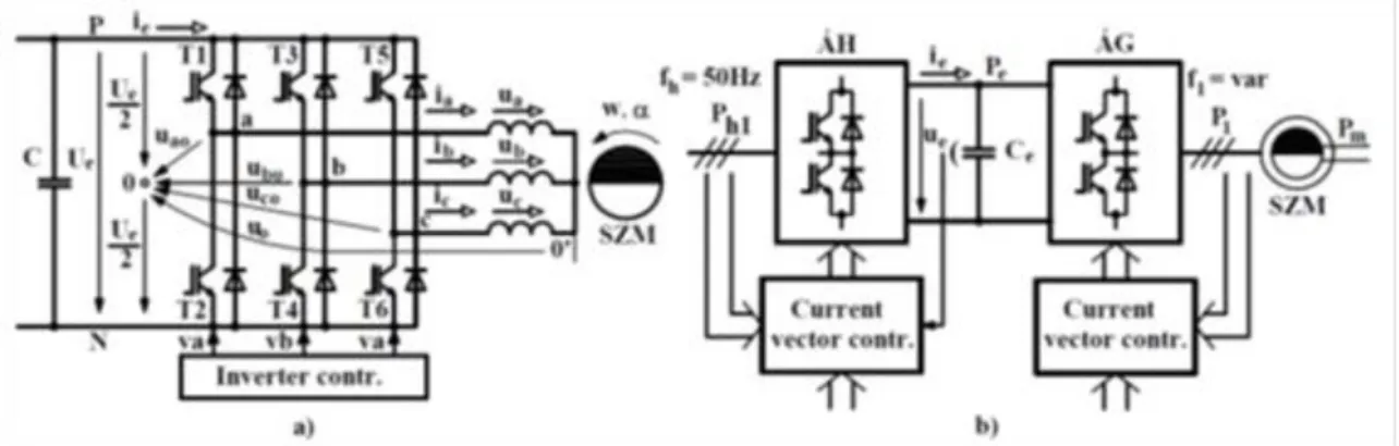
The energy flow is possible in both direction, if the DC circuit is capable of it. In the case of the intermediate DC link versions it depends on the way how the Ue=const. DC voltage is generated (chapter 7). In the most modern version (Fig.4.9.b.) either the machine-side converter ÁG or the line-side converter ÁH are VSI type. In this way the power can flow in both directions. In the simplest case ÁH is a diode bridge, when only motor mode operation is possible. In motor mode (driving mode) the mean value of the DC current is positive Iek>0, while in generator (brake) mode it is negative Iek<0. Assuming lossless energy conversion chain the power mean values are (with the notation in Fig. 4.9.b.):

2.3. Current vector controls

The aim is to track the īa current reference vector (determined by the driving task) without error . By a non-continuous state VSI it is not possible. The derivative of the current error vector corresponding to the ū=ū(k) voltage vector can be expressed using the ū=Rī+Ld·dī/dt+ūp voltage equation (derived from Fig.3.2.b.), and considering expression:

(4.16.a,b)

The ē fictive voltage vector (using approximation), means the necessary continuous voltage vector for the errorless tracking: ī=īa. In every instant the current controller can select from 7 kinds of ū(k) voltage vectors (4.14). If the selection is optimal, then the ī current vector tracks the īa reference with small error (ī oscillates around īa).

Similarly to the chopper-fed DC drive (Fig.2.20.) two kinds of current vector control spread widely in practice:

the PWM modulator based and the hysteresis control. In the PWM modulator based current vector control (Fig.4.11.a.) the PWM VSI has a PWM modulator, and the current controller acts through this modulator indirectly. The hysteresis current vector controllers (Fig. 4.11.b.) control the PWM VSI directly. In Fig.4.7.a.,b.

PWM modulator based version is assumed.

(35)

Fig.4.11. Current vector control methods. a. PWM modulator based controller, b. Hysteresis controller.

2.3.1. PWM modulator based current vector controls

The PWM modulator based current vector control (Fig.4.11.a.) has more versions, depending on in which coordinate system the components of the ī current vector are controlled, and which are the input signals of the PWM modulator. If the SZI controllers control the dq components, then the two versions in Fig.4.12.a.,b., if the abc components (phase currents), then the two versions in Fig. 4.12.d.,e. are possible. The SZI current controllers are PI type in the practice. Fig.4.12.c. presents how the components d-q are produced. The control signals (with index v) control space-vector PWM modulator in the a,e versions and three-phase PWM modulator in the b,d versions. The necessity of the coordinate transformations is obvious in all cases.

Fig.4.12. Block diagrams of the PWM modulator based current vector controls. a,b,c. Controllers in dq coordinates, d,e. Controllers in abc coordinates.

Le‟s examine the versions in Fig.4.12.a. and Fig. 4.12.d. in a little bit more detail.

Current vector control with dq components, by space-vector PWM (SPWM) (Fig.4.12.a.). The detailed block diagram of this version is in Fig.4.13.

The blocks SZID and SZIQ are usually PI type current controllers, their outputs (uvd and uvq) form a control vector , which is proportional to the ū1 fundamental voltage vector of the PWM inverter (the motor), if the fISZM switching frequency is large enough. According to the experience, if fISZM>20f1 then ū1=Kuūv. As a synchronous machine is investigated, the maximal value of f1 is determined by the maximal speed (n=n1=f1/p).

In practice: f1max≤100Hz, so with fISZM≥2kHz the above proportionality is well correct. The input signals of the SPWM are the uv amplitude and αv angle of the ūv control vector, its output signals are the two-level va, vb, vc inverter control signals. In practice, the SPWM is operating in sampled mode, the sample frequency is equal to the fISZM frequency.

(36)

Fig.4.13. Current vector control with dq components, by SPWM.

Fig.4.14. Voltage vectors. a. Creation of ū1(n) in sector 1, b. The 60° wide sectors.

Using sampled SPWM in the nth sample period with the control vector

(4.17.a,b,c)

fundamental voltage vector is prescribed. Ku is the voltage gain factor of the SPWM controlled VSI. The ū1(n) vector can be produced by switching on the neighbour three ū(k) voltage vectors (Fig. 4.14.b) for proper time interval. In the time instant presented in Fig.4.14.a. the ū1(n) is in the sector 1 of 60° degree.

Here ū(1), ū(2) and ū(7) are the three neighbour vectors. The ū1(n) vector is developed as the time weighted mean value of these vectors:

(4.18)

Where τ1n+τ2n+τ7n=τ=const. is the sampling period, b1n+b2n+b7n=1 is the sum of the duty cycles. The b1n, b2n and b7n

duty cycles can be derived from the geometric considerations based on Fig.4.14.a.:

(4.19.a,b,c)

Where U1max is the possible maximum fundamental peak value, which is according to Fig.4.14.a. is:

(37)

(4.20)

The function of the duty cycles in sector 1 is presented in Fig.4.15. for 0,8U1max amplitude ū1 fundamental voltage. b1n and b2n are proportional to the prescribed u1(n)=0,8U1max amplitude, the b1n/b2n ratio depends on the α1(n) angle. The switching between the 3 possible vectors can be done in two ways (Table 4.2.).

Fig.4.15. The angle dependency of the duty cycles in sector 1 with u1(n)/U1max=0,8.

Table 4.2. Switching methods in sector 1.

Method I. Metho

d II.

k 1 2 7 1 2 7 1 2 7 1 2 7P 2 1 7N 1 2 7P

sample n n+1 n+2 n n+1 n+2

There is one double switch at method I. in every sampling period, even by 7P or by 7N the ū(7)=0 voltage vector is produced. It is eliminated using method II. by the periodical changing of the switching order of ū(1), ū(2), 7P and 7N. Considering Table 4.2. and Fig.4.14.b. it can be established, that at method I. 4, at method II. 3 switchings correspond to one sampling period. I.e. using method II. the switching number can be reduced to ratio ¾ and also the switching loss proportional to it, comparing with method I.

The operation of the SPWM is investigated in sector 1, but it operates in the other sectors similarly.

Current vector control with abc phase quantities, by three-phase PWM modulator (3-Ph PWM) (Fig.4.12.d.).

(38)

Fig.4.16. Current vector control with abc phase quantities, by 3-Ph PWM.

Fig.4.17. Three-phase analogue PWM modulator

Fig.4.18. Operation of the analogue PWM modulator (fΔ/f1=9).

The SZIA, SZIB and SZIC are usually PI type current controllers, their output signals are the uva, uvb and uvc

phase control signals (modulating signals). Processing them the 3-Ph PWM generates the two-level control signals va, vb, vc for the inverter. The 3-Ph PWM consists of 3 one-phase modulator, but the carrier wave of the modulators (uΔ) is common (Fig.4.17.).

Operation of the analogue PWM modulator is demonstrated in Fig.4.18. for phase a. (Nowadays digital modulators implemented by counters are applied.) While uva>uΔ, then va=H (high level), phase a is on the P bar:

ua0=+Ue/2. When uva<uΔ, then va=L (low level), phase a is on the N bar: ua0=-Ue/2. There exist fΔ/f1=const.

synchronous modulation and, fΔ=const., fΔ/f1=var. asynchronous modulation. It can be proved, that in steady- state in the output voltage of the inverter besides the fundamental component with frequency f1 upperharmonics with frequencies fΔ±2f1, fΔ±4f1,…, 2fΔ±f1, 2fΔ±3f1,… also appear.

The synchronous machine thanks to its Ld synchronous inductance is very good filter for the current and the torque. It is demonstrated in Fig.4.19. drawn according to Fig. 4.2. Here Δū and Δī are the resultants of the upperharmonics: