in a diffusive ratio-dependent predator–prey system with linear stocking rate of prey species

(1)

Temporal and spatial patterns

in a diffusive ratio-dependent predator–prey system with linear stocking rate of prey species

Wanjun Li

¹

, Xiaoyan Gao

²

and Shengmao Fu

^B²

1School of Mathematics and Statistics, Longdong University, Qingyang, 745000, P.R. China

2School of Mathematics and Statistics, Northwest Normal University, Lanzhou, 730070, P.R. China

Received 25 July 2018, appeared 30 October 2019 Communicated by Ferenc Hartung

Abstract. The ratio-dependent predator–prey model exhibits rich interesting dynamics due to the singularity of the origin. It is one of prototypical pattern formation models.

Stocking in ratio-dependent predator–prey models is relatively an important research subject from both ecological and mathematical points of view. In this paper, we study the temporal, spatial patterns of a ratio-dependent predator–prey diffusive model with linear stocking rate of prey species. For the spatially homogeneous model, we derive conditions for determining the direction of Hopf bifurcation and the stability of the bifurcating periodic solution by the center manifold and the normal form theory. For the reaction-diffusion model, firstly it is shown that Turing (diffusion-driven) instability occurs, which induces spatial inhomogeneous patterns. Then it is demonstrated that the model exhibits Hopf bifurcation which produces temporal inhomogeneous patterns.

Finally, the non-existence and existence of positive non-constant steady-state solutions are established. We can see spatial inhomogeneous patterns via Turing instability, temporal periodic patterns via Hopf bifurcation and spatial patterns via the existence of positive non-constant steady state. Moreover, numerical simulations are performed to visualize the complex dynamic behavior.

Keywords: ratio-dependent, stocking rate, Hopf bifurcation, Turing instability, steady- state, pattern.

2010 Mathematics Subject Classification: 92D25, 35K57, 35B35.

1 Introduction

One of important ecological fields is the dynamics between predators and prey. Since the first differential equation model of predator–prey type was found by Lotka [18] and Volterra [27] in 1920s, various kinds of predator–prey models have been proposed and studied. Some of these models are those with Holling types I, II, III and IV functional responses and have

BCorresponding author. Email: fusm@nwnu.edu.cn

(2)

been intensively investigated, for example in [6,13,23,30]. The Holling type II (or Michaelis–

Menten) model is of the form du

dt =ru

1− ^u K

− ^c¹^uv m+u, dv

dt =v

−d+ ^c²^u m+u

,

(1.1)

where u,v stand for prey and predator density, respectively. r,K,c₁,m,c₂,d are positive constants that stand for prey intrinsic growth rate, carrying capacity, capturing rate, half capturing saturation constant, conversion rate, predator death rate, respectively. While many of the mathematicians working in mathematical biology may regard these as important contri- butions that mathematics had for ecology, they are very controversial among ecologists up to this day. Indeed, some ecologists may simply view it as a problem [2,4], because they are not in line with many field observations [2,3,12].

Recently there is a growing evidences [3,5,10] that in some situations, especially when predator have to search for food (and therefore have to share or compete for food), a more suitable general predator–prey theory should be based on the so called ratio-dependent theory, which can be roughly stated as that the per capita predator growth rate should be a function of the ratio of prey to predator abundance. This is supported by numerous field and laboratory experiments and observations [2,3]. Compared with Holling type functional responses, the ratio-dependent type functional response is more suitable to describe the inter- action between the predator and prey.

The ratio-dependent predator–prey model have been studied by many researchers and very rich dynamics have been observed, see [1,9,24,26,32] and references therein. Now, we focus our attention on the following ratio-dependent predator–prey model

du dt =ru

1− ^u

K

− ^c¹^uv mv+u, dv

dt =v

−d+ ^c²^u mv+u

.

(1.2)

The term _mv^c¹₊^u_u is called the ratio-dependent Holling type II functional response, and is derived from p(u/v), where p is the Holling type II prey-dependent functional response defined by

p(u) = ^c¹^u

m+u. (1.3)

We refer to [11] and the references therein for the study of the predator–prey system (1.1).

However, more realistic and suitable predator–prey systems should rely on the ratio-dependent functional responses. Roughly speaking, the per capita predator growth rate should be a function of the ratio of prey to predator abundance. Hence, the prey-dependent functional response p(u) given in (1.3) would be replaced by the ratio-dependent functional response p(u/v).

The dynamics of the model (1.2) has been studied extensively [7,14,29,31]. These re- searches on the ratio-dependent predator–prey model (1.2) revealed rich interesting dynamics such as deterministic extinction, existence of multiple attractors, and existence of a stable limit cycle. Especially, it was shown in [7], [14], and [29] that the model (1.2) has very complicated dynamics close to the origin: There exist numerous kinds of topological structures in a neigh- borhood of the origin, including parabolic orbits, elliptic orbits, hyperbolic orbits, and any combination thereof, depending on the different values of parameters.

(3)

In realistic ecology, the activities of harvesting or stocking often occur in fishery, forestry, and wildlife management. For example, certain number of animals are removed per year by hunting. It leads one to add harvesting rates or stocking rates into some models, see [8,20,33].

In this paper, we insert a linear stocking rate δ of prey into the first equation (1.2) and study the bifurcation dynamics of the following ratio-dependent predator–prey system with linear stocking rate

du dt =ru

1− ^u

K

− ^c¹^uv

mv+u +δu, dv

dt =v

−d+ ^c²^u mv+u

.

(1.4)

In [19], M. Lei investigated the permanence of a class of Holling III-Tanner predator–prey diffusion system with stocking rate and time delay, the existence of positive periodic solution by using comparability theorem, coincidence degree theory. They obtained the sufficient conditions which guarantee permanent of the system and existence of the positive periodic solution of the periodic system. In [28], Z. Wang et al. considered a nonautonomous predator–

prey system with Holling III functional responses and stocking rate. They proved that the system is uniformly permanent under suitable condition. Furthermore, sufficient criteria are established for existence, uniqueness and global asymptotic stability of periodic solution by establishing Lyapunov function. Anorexia predator–prey system under constant stocking rate of prey is discussed. The local behaviour and global behaviour of feasible equilibrium points were studied and the conditions of the existence and non-existence of limit cycle are obtained.

For simplicity, using the scaling: u →u/K,v →mv/K,t →rt, one can change the model (1.4) into the following equivalent system

du

dt =_u(₁−u)− ^αuv u+v+_hu, dv

dt =v

−γ+ ^βu u+v

,

(1.5)

whereα=c₁/(rm),β= c₂/r,γ= d/r,h=δ/r.

When the densities of the prey and predator are spatially inhomogeneous in a bounded domain, and the prey and predator move randomly-described as Brownian random motion, we need consider the following reaction-diffusion model corresponding model (1.5). In this paper, we investigate the temporal, spatial and temporospatial patterns of the following diffusive ratio-dependent predator–prey model with prey stocking

∂u

∂t −d₁4u= u(1−u)− ^αuv

u+v +hu, x∈_Ω, t>0,

∂v

∂t −d₂4v =v

−γ+ ^βu u+v

, x∈_Ω, t>0,

∂u

∂ν

= ^∂v

∂ν

=_0, x∈∂Ω, t >_0,

u(x, 0) =u₀(x), v(x, 0) =v₀(x), x∈_Ω,

(1.6)

where Ω ⊂ _Rⁿ(n ≥ 1) is a smooth bounded domain, ν is the outward unit normal vector on ∂Ω. d₁,d₂,α,β,γ,h are all positive constants. u₀(x) and v₀(x) are nonnegative smooth functions andu₀(x) +v₀(x)>_0.

(4)

To study the stationary patterns, we need consider the steady-state problem associated with (1.6)

−d₁4u=u(1−u)− ^αuv

u+v+hu, x∈ _Ω,

−d₂4v=v

−γ+ ^βu u+v

, x∈ _Ω,

∂u

∂ν = ^∂v

∂ν =0, x∈ _∂Ω.

(1.7)

This paper is organized as follows. In Section2, we investigate the existence, direction and stability of the Hopf bifurcation for the model (1.5) by applying the Poincaré–Andronov–Hopf bifurcation theorem. In Section 3, we first consider the Turing (diffusion-driven) instability of the reaction-diffusion model (1.6) when the spatial domain is a bounded interval, which will produce spatial inhomogeneous patterns. Then we study the existence and direction of Hopf bifurcation and the stability of the bifurcating periodic solution, which is a spatially inhomogeneous periodic solution of (1.6). In Section 4, we first give a priori estimates for the positive steady-state solutions of the model (1.7), then consider the existence and non- existence of positive non-constant steady states of (1.7). Moreover, numerical simulations are presented to verify and illustrate the above theoretical results. The paper ends with a brief discussion.

2 Dynamics of the ODE model

Let

f₁(u,v) =u(1−u)− ^αuv

u+v+hu, f₂(u,v) =v

−γ+ ^βu u+v

.

It is easy to know that model (1.5) has a free equilibrium (1+h, 0) and the unique positive equilibriumU^∗ = (u^∗,v^∗) = ^αγ⁺^β⁽¹⁺^h⁻^α⁾

β , ^β⁻_γ^γ u^∗

if and only if (H₁)

β>γ, h>max

0,α−1− ^αγ β

.

In this section, we mainly discuss the existence, direction and stability of the Hopf bifurcation in the model (1.5). The Jacobian matrix of model (1.5) atU^∗ as follows

J =

a₁₁ a₁₂ a₂₁ a₂₂

, where

a₁₁ = (α−h−1)β²−αγ²

β² , a₁₂ =−^αγ² β²

<0,

a₂₁ = (γ−β)²

β >0, a22 = (γ−β)γ β <0.

The characteristic polynomial is

P(λ) =λ²−_Υλ+_Θ, where

Υ=α−γ−h−1+ ^γ

2

β²(β−α), Θ= ^γ(β−γ)(αγ+β(1+h−α))

β² .

For the Jacobian matrix J, we have the following conclusions.

(5)

Lemma 2.1.

(1) Θ>0if(H₁)holds.

(2) a₁₁ >0if the following assumption holds (H₂)

h<α−1−^αγ

2

β² .

By the standard linearization method, we can easily prove the following theorem.

Theorem 2.2. Free equilibrium (1+h, 0) of (1.5) is locally asymptotically stable if β < γ and is unstable if β>γ.

Theorem 2.3. Suppose that(_H₁)holds. The unique positive equilibrium U^∗of (1.5)is locally asymptotically stable if

(H31)

h>α−γ−1+ ^γ

2

β²(β−α),^h0

and is unstable if

(H₃₂) h<h₀.

To analyze the Hopf bifurcation of (1.5) occurring atU^∗, we takehas the bifurcation param- eter. In fact, h plays an important role in determining the stability of the interior equilibrium and the existence of Hopf bifurcation. Clearly,h₀ >0 if and only if

(H₄) (γ+1)β²+αγ²<αβ²+βγ²).

Letλ(h) =φ(h)±iϕ(h)be a pair of complex roots ofP(λ) =0 whenhnearh₀. Then φ(h) = ^Υ

2, ϕ(h) = ¹ 2

q

−4a₁₂a₂₁−(a₁₁−a₂₂)²_. Furthermore, we can verify

φ(h₀) =0, φ⁰(h₀) =−¹ 2 <0.

This means that the transversality condition holds. By the Poincaré–Andronov–Hopf bifurcation theorem [17], we know that (1.5) undergoes a Hopf bifurcation atU^∗ ashpasses through theh0.

To understand the detailed property of the Hopf bifurcation, we need a further analysis for the normal form of the model (1.5). Being more specific, we use the framework [16] to analysis the direction and stability of the Hopf bifurcation of the model (1.5).

We translate the positive equilibriumU^∗to the origin by the transformationue= u−u^∗,ve= v−v^∗. For the sake of convenience, we still denoteueandvebyuandv. Thus, the local system (1.5) is transformed into

du

dt = (u+u^∗)(1−(u+u^∗))− ^α(u+u^∗)(v+v^∗)

(u+u^∗) + (v+v^∗)+h(u+u^∗), dv

dt = (v+v^∗)

−γ+ ^β(u+u^∗) (_u+_u^∗) + (_v+_v^∗)

.

(2.1)

(6)

Rewrite the system (2.1) as





 du

dt dv dt





= J u

v

+

f(u,v,δ) g(u,v,δ)

, (2.2)

where

f(u,v,δ) =a₁u²+a₂uv+a₃v²+a₄u³+a₅u²v+a₆uv²+a₇v³+· · · , g(u,v,δ) =b₁u²+b₂uv+b₃v²+b₄u³+b₅u²v+b₆uv²+b₇v³+· · · , and

a₁=−1+ ^αv

∗2

(u^∗+v^∗)³^, ^a² =− ^2αu

∗v^∗

(u^∗+v^∗)³^, ^a³= ^αu

∗2

(u^∗+v^∗)³^, ^a⁴ =− ^αv

∗2

(u^∗+v^∗)⁴^, a5= ^2αu

∗v^∗−αv^∗²

(u^∗+v^∗)⁴ ^, ^a⁶ = ^2αu

∗v^∗−αu^∗²

(u^∗+v^∗)⁴ ^, ^a⁷=− ^αu

∗2

(u^∗+v^∗)⁴^, b₁=− ^βv

∗2

(u^∗+v^∗)³^, ^b² = ^2βu

∗v^∗

(u^∗+v^∗)³^, ^b³=− ^βu

∗2

(u^∗+v^∗)³^, ^b⁴ = ^βv

∗2

(u^∗+v^∗)⁴^, b₅= ^βv

∗2−2βu^∗v^∗

(u^∗+v^∗)⁴ ^, ^b⁶ = ^βu

∗2−2βu^∗v^∗

(u^∗+v^∗)⁴ ^, ^b⁷= ^βu

∗2

(u^∗+v^∗)⁴^. Set the matrix

P:=

N 1

M 0

, where M=−^a²¹

ϕ , N= ^a²²_2ϕ⁻^a¹¹. It is easy to obtain that P⁻¹JP=_Φ(h):=

φ(h) −ϕ(h) ϕ(h) φ(h)

. Let

M₀ := M|_h₌_h₀, N₀:= N|_h₌_h₀, ϕ₀:= ϕ(h₀). (2.3) By the transformation(u,v)^T =P(x,y)^T, the system (2.2) becomes





 dx

dt dy dt





 =_Φ(h) x

y

+

f¹(x,y,h) g¹(x,y,h)

, (2.4)

where

f¹(x,y,h) = ¹

Mg(Nx+y,Mx,h)

= N²

Mb₁+Nb₂+Mb₃

x²+ 2N

M b₁+b₂

xy+ ^b¹ My² +

N³

Mb₄+N²b₅+N Mb₆+M²b₇

x³+ 3N²

M b₄+2Nb₅+Mb₆

x²y +

3N Mb₄+b₅

xy²+ ^b⁴

My³+· · · ,

(7)

g¹(x,y,h) = f(Nx+y,Mx,h)− ^N

Mg(Nx+y,Mx,h)

=

N²a₁+N Ma₂+M²a₃− ^N³

Mb₁−N²b₂−N Mb₃

x² +

2Na₁+Ma₂− ^2N

2

M b₁−Nb₂

xy+

a₁− ^N Mb₁

y² +

N³a₄+M³a7+N²Ma5+N M²a6− ^N

4

Mb₄−N³b5−MN²b6+N M²b7

x³ +

3N²a₄+2N Ma₅+M²a₆− ^3N

3

M b₄−2N²b₅−N Mb₆

x²y +

3Na₄+Ma₅− ^3N

2

M b₄−Nb₅

xy²+

a₄− ^N Mb₄

y³+· · · . The polar coordinates form of (2.4) is as the following

˙

τ=φ(h)τ+a(h)τ³+· · · _,

θ˙ = ϕ(h) +c(h)τ²+· · · , (2.5) then it follows from the Taylor expansion of (2.5) atδ=δ₀that

˙

τ= φ⁰(h₀)(h−h₀)τ+a(h₀)τ³+o((h−h₀)²τ, (h−h₀)τ³, τ⁵),

θ˙= ϕ(h₀) +ϕ⁰(h₀)(h−h₀) +c(h₀)τ²+o((h−h₀)²_, (h−h₀)τ², τ⁴)_. ^(2.6) In order to determine the stability of the Hopf bifurcation periodic solution, we need to cal- culate the sign of the coefficienta(h0), which is given by

a(h₀) = ¹ 16

f_xxx¹ + f_xyy¹ +g¹_xxy+g¹_yyy + ¹

16ϕ₀ h

f_xy¹ (f_xx¹ + f_yy¹ )−g¹_xy(g¹_xx+g¹_yy)− f_xx¹ g¹_xx+ f_yy¹ g¹_yyi ,

(2.7)

where all partial derivatives are evaluated at the bifurcation point(x,y,h) = (0, 0,h₀), and f_xxx¹ (0, 0,h₀) =6

N₀³

M₀b₄+N₀²b₅+N₀M₀b₆+M₀²b₇

, f_xyy¹ (0, 0,h₀) =2 3N₀

M₀b₄+b₅

, g¹_xxy(0, 0,h₀) =2

3N₀²a₄+2N₀M₀a₅+M²₀a₆−^3N

03

M₀ b₄−2N₀²b₅−N₀M₀b₆

, g¹_yyy(0, 0,h₀) =6

a₄− ^N⁰ M₀b₄

, f_xx¹ (0, 0,h₀) =2 N₀²

M₀b₁+N₀b₂+M₀b₃

, f_xy¹ (0, 0,h0) = ^2N⁰

M₀b₁+b2, f_yy¹ (0, 0,h0) = ² M₀b₁, g¹_xx(0, 0,h₀) =2

N₀²a₁+N₀M₀a₂+M²₀a₃− ^N

03

M0

b₁−N₀²b₂−N₀M₀b₃

, g¹_xy(0, 0,h₀) =2N₀a₁+M₀a₂− ^2N

02

M₀ b₁−N₀b₂, g¹_yy(0, 0,h₀) =2

a₁− ^N⁰ M₀b₁

. Thus, we can determine the value and sign of a(h₀)in (2.7).

Recall thatσ2 =−^a⁽^h⁰⁾

φ⁰(h0) andφ⁰(h0) =−¹₂ <0, form the Poincaré–Andronov–Hopf bifurcation theorem, we can summarize our results as follows.

(8)

Theorem 2.4. Suppose that (H₁)and(H₄)hold. Then model (1.5) undergoes a Hopf bifurcation at U^∗ when h= h0.

(1) The direction of the Hopf bifurcation is subcritical and the bifurcated periodic solutions are or- bitally asymptotically stable if a(h₀)<0;

(2) The direction of the Hopf bifurcation is supercritical and the bifurcated periodic solutions are unstable if a(h₀)>0.

To illustrate Theorem2.4, we give some simple numerical examples.

Example 2.5. (1) We choose the coefficients in the system (1.5) as follows

α=4, β=1, γ=0.5. (2.8)

It is easy to see that(H₄)holds and the critical point h₀ = 1.75. Set h = 1.5, thenU^∗ = (0.5, 0.5),Υ=0.25>0,Θ=0.125>0, i.e. (_H₁),(_H₃₂)hold and soU^∗ is unstable.

Set h = 2.5 and the parameters in (2.8) satisfy (_H₁)_{. Then}_U^∗ = (_{1.5, 1.5})_, _Υ = −0.75<

0,Θ = 0.375 > 0, by Theorem 2.3, U^∗ is locally asymptotically stable. Besides, a(h₀) ≈

−1.407 < 0 and σ₂ ≈ −1.407 < 0. By Theorem 2.4, Hopf bifurcation occurs at h = h₀, the Hopf bifurcation is subcritical and the bifurcating periodic solutions are stable.

(2) If we choose

α=1.7, β=1, γ=0.4. (2.9)

It is easy to see that(_H₄)holds and the critical pointh₀ =0.188,U^∗ = (0.168, 0.252), a(δ₀)≈ 0.227> 0 and σ2 ≈ 0.227 > 0. By Theorem 2.4, Hopf bifurcation occurs ath = h0, the Hopf bifurcation is supercritical and the bifurcating periodic solutions are unstable.

3 Turing instability and bifurcations in the reaction-diffusion model

In this section, we mainly discuss the stability of positive equilibrium and the existence, stability and direction of the Hopf bifurcation for the reaction diffusion system (1.6). For simplicity, we shall take the spatial domainΩas the one-dimensional intervalΩ= (0,π), and consider

u_t−d₁u_xx=u(1−u)− ^αuv

u+v +hu, x ∈(0,π), t>0, v_t−d₂v_xx=v

−γ+ ^βu u+v

, x ∈(0,π), t>0, ux(0,t) =ux(π,t) =vx(0,t) =vx(π,t) =0, t >0,

u(x, 0) =u₀(x)_, v(x, 0) =v₀(x)_, x ∈(_0,π)_.

(3.1)

It is well known that the operatoru → −u_xxwith no-flux boundary condition has eigenvalues and eigenfunctions as follows:

µ₀=0, φ₀ = r1

π, µ_i =i², φ_i(x) = r2

πcosix, for i=1, 2, 3, . . .

(9)

3.1 Diffusive effects on the interior equilibrium point Theorem 3.1. Assume that the conditions(H1)and h>α−1− ^αγ²

β² hold. Then the unique positive equilibrium U^∗ in(3.1)is uniformly asymptotically stable.

Proof. Let D = _diag(d₁,d₂)_, U = (u,v) _, L = D4+J_U(U^∗). Then the linearized system of (3.1) atU^∗ is

U_t = LU, (3.2)

and the eigenvalues of the operatorLare the eigenvalues of the matrix−µ_iD+J_U(U^∗),∀i≥1.

The characteristic equation of−µ_iD+J_U(U^∗)is

ϕ_i(λ),|λI+µ_iD−J_U(U^∗)|= λ²+A_iλ+B_i =0, where

A_i = µ_i(d₁+d₂)−_Υ, B_i = µ²_id₁d₂−a₁₁µ_id₂−a₂₂µ_id₁+_Θ, andΥ,Θbe defined as in the Section 2.

Ifh>α−1−^αγ²

β² , thena₁₁<0, A_i >0 andB_i >0. The rootsλ_i,1 andλ_i,2of ϕ_i(λ) =0 all have negative real parts.

We claim that there exists a positive constant ¯δsuch that

Re{λ_i,1}, Re{λ_i,2} ≤ −δ,^¯ ∀i≥1. (3.3) In fact, letλ=µ_iζ, then

ϕ_i(λ) =µ²_iζ²+_A_iµ_iζ+_B_i, ^ϕi(ζ)_, and

ilim→_∞

ϕ_i(ζ) µ²_i

=ζ²+ (d₁+d₂)ζ+d₁d₂, ^ϕ(ζ).

Notice that ϕ(ζ) =0 has two negative roots −d₁ and−d₂. Thus, Re{ζ₁}, Re{ζ₂} ≤ −d =

−min{d₁,d2}. By continuity, there exists an i0 such that the two roots ζ_i,1,ζ_i,2 of ϕ_i(ζ) = 0 satisfy Re{ζ_i,1}, Re{ζ_i,2} ≤ −d/2, ∀i≥i₀. In turn, Re{λ_i,1}, Re{λ_i,2} ≤ −d/2 , ∀i≥i₀.

Let

max{Re{λ_i,1}, Re{λ_i,2}}= −η.

Thenη>0, and (3.3) holds for ¯δ=min{η,d/2}.

This implies that the spectrum of L, which consists of eigenvalues, lies in {Reλ ≤ −δ^¯}, and uniform stability ofU^∗ follows [15]. This completes the proof.

From Lemma2.1and Theorem2.3, we know that the interior equilibriumU^∗ of the ODE model (1.5) is locally asymptotically stable if (H₃₁) holds, that is, Υ < 0. To investigate the Turing instability of the spatially homogeneous equilibrium U^∗ of the diffusive model (3.1), we need look for the condition of diffusion-driven instability under the assumption(H31). It is well known that the positive equilibriumU^∗ of (3.1) is unstable if ϕ_i(λ) =0 has at least one root with positive real part.

For the sake of convenience, define

φ(µ_i)_:= B_i =µ²_id₁d₂−(a₁₁d₂+a₂₂d₁)µ_i+_Θ,

(10)

which is a quadratic polynomial with respect to µ_i. It is necessary to determine the sign of φ(µ_i). Clearly, ifφ(µ_i)<0, then ϕ_i(λ) =0 has two real roots in which one is positive and the other is negative. Notice that if

G(d₁,d₂)_:=a₁₁d₂+a₂₂d₁ >_0, thenφ(µ_i)will take the minimum value

min

µi

φ(µ_i) =_Θ− (a₁₁d₂+a₂₂d₁)² 4d₁d₂ <0 at the critical valueµ^∗ >0, whereµ^∗ = ^a¹¹^d_2d²⁺^a²²^d¹

1d2 . Define the ratioρ=_d₂_/d₁_and

Λ(d₁,d₂) = (a₁₁d₂+a₂₂d₁)²−4d₁d₂Θ

=a²₁₁d²₂+2(2a₁₂a₂₁−a₁₁a22)d₁d2+a²₂₂d²₁. Then

Λ(d₁,d2) =0⇔ a²₁₁ρ²+2(2a₁₂a₂₁−a₁₁a22)ρ+a²₂₂=0, G(d₁,d₂) =0⇔ρ =−^a²²

a₁₁ ≡ρ^∗. Recall thatΘ>0 anda₁₂<0, a₂₁>0, we have

4(2a₁₂a₂₁−a₁₁a₂₂)²−4a²₁₁a²₂₂=16a₁₂a₂₁(a₁₂a₂₁−a₁₁a₂₂)>0.

Therefore,Λ(d₁,d₂) =0 has two positive real roots ρ₁= −(2a₁₂a₂₁−a₁₁a22) +2p

a₁₂a₂₁(a₁₂a₂₁−a₁₁a22)

a²₁₁ ,

ρ₂= −(2a₁₂a₂₁−a₁₁a₂₂)−2p

a₁₂a₂₁(a₁₂a₂₁−a₁₁a₂₂)

a²₁₁ ,

and 0< ρ₂ < ρ^∗ < ρ₁. Moreover, if d₂/d₁ > ρ₁, then minφ(µ_i) < 0, G(d₁,d₂) < 0, andU^∗ is unstable. It follows from Theorem 2.4 that the Turing instability occurs. Based on the above analyze, we have the following Turing instability result.

Theorem 3.2. Assume that the conditions(_H₁)and(_H₃₁)hold(in the case U^∗ is stable with respect to the local model(1.5)). Then there exists an unbounded region

T:= {(d₁,d₂):d₁ >0, d₂>0, d₂ >ρ₁d₁}

forρ₁ >0, such that, for any(d₁,d₂)∈ T, U^∗ is unstable with respect to the reaction-diffusion model (3.1), that is, Turing instability occurs.

Example 3.3. (1) We choose the coefficients of the model (3.1) as follows

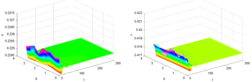
α=_1.5, β=_1, γ=_0.35, _h=_0.2, _d₁=_0.015, _d₂=_0.25. _(3.4) It is easy to see that the parameters in (3.4) satisfy (H₁) and Υ = −0.11125 < 0, i.e.

(_H₃₁) holds. The unique positive equilibrium point U^∗ ≈ (0.225, 0.4179) in (1.5) is locally

(11)

Figure 3.1: Stable behaviour withd₁ =0.015,d2=0.25 for the model (3.1).

asymptotically stable. Furthermore,ρ₁≈ _{18.86 and}d₂−ρ₁d₁ ≈ −_0.0329<_{0, so}U^∗ in (3.1) is uniformly asymptotically stable (see Fig. 3.1).

(2) Choose

α=1.5, β=1, γ=0.35, h=0.2, d₁ =0.015, d₂ =0.5. (3.5) In (3.5), we only change a diffusion coefficient compared with (3.4). In the case,ρ₁ ≈18.862 andd₂−ρ₁d₁ ≈0.217> 0. By Theorems 2.3,3.2, we know thatU^∗ ≈ (0.225, 0.4179)_{is stable} with respect to the local model (1.5), and unstable for the diffusive system (3.1). This means that the Turing instability occurs in (3.1) (see Fig.3.2).

Figure 3.2: Turing instability withd₁ =0.015,d2=0.5 for the model (3.1).

(3) Choose

α=1.7, β=3, γ=1.2, h=0.2, d₁ =0.01, d₂ =0.5. (3.6) In (3.6), all coefficients are changed but satisfy(H₁)and(H₃₁). Thus, U^∗ = (0.18, 0.27)in (1.5) is locally stable. In this case, ρ₁ ≈ 15.65 and d₂−ρ₁d₁ ≈ 0.3435 > 0. By Theorem 3.2, Turing instability occurs in the diffusive system (3.1) (see Fig.3.3).

Remark 3.4. Via numerical simulations, we can see that the model exhibits spatiotemporal complexity of pattern formation, including stripe, stripe-hole and hole Turing patterns.

For example, in (3.1), fix

α=1.5, β=1, γ=0.35, h=0.2, d₁ =0.01, d₂ =0.62. (3.7) By numerical simulation results, we can observe the stripe-hole pattern ofuin the model (3.1) (see Fig.3.4). Changing the diffusion coefficientsd₁ =0.015,d₂ =0.3 in (3.7), hole pattern can be obtained (see Fig.3.5).

(12)

Figure 3.3: Turing instability withd₁=0.01,d2 =0.5 for the model (3.1).

0.05 0.1 0.15 0.2 0.25 0.3 0.35 0.4 0.45

Figure 3.4: Stripe-hole pattern of u in the model (3.1).

0.1 0.15 0.2 0.25

0.05 0.1 0.15 0.2 0.25 0.3

Figure 3.5: Hole pattern ofuin the model (3.1).

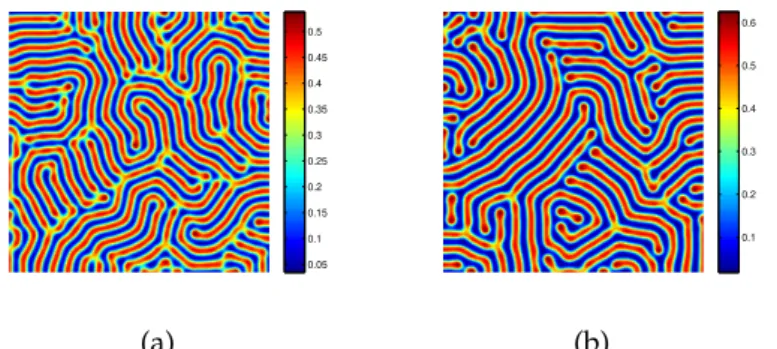
If we fix

α=3, β=1.3, γ=0.2, h=1.8, d₁=0.01,

we can see that pattern with d₁ = 0.25 is similar to the one with d₁ = 0.45, they are all stripe patterns in (Fig.3.6). Fig. 3.6(a) consists of blue stripe on a red background, i.e., the prey is isolated zones with low population density. While (b) consists of red stripe on a blue background, i.e., the prey is isolated zones with high population density.

3.2 Diffusive effects on the bifurcation limit cycle

In this subsection, we seek for the related Hopf bifurcation points and consider the stability of the bifurcating periodic solutions of model (3.1) with spatial domain(0,π). In order to use framework of the Hopf bifurcation theory [16], we need to complete the following three steps.

Step 1. Linearization analysis.

For (3.1), we introduce the perturbation u = uˆ+u^∗,v = vˆ+v^∗, and still denote (u, ˆˆ v)_by

(13)

0.05 0.1 0.15 0.2 0.25 0.3 0.35 0.4 0.45 0.5

(a)

0.1 0.2 0.3 0.4 0.5 0.6

(b)

Figure 3.6: Stripe pattern ofu in the model (3.1).

(u,v). Then

u_t−d₁u_xx= (u+u^∗)(₁−(u+u^∗))− ^α(u+u^∗)(v+v^∗)

(u+u^∗) + (v+v^∗)+h(u+u^∗)_, x∈(_0,π)_, t>_0, v_t−d₂v_xx= (v+v^∗)

−γ+ ^β(u+u^∗) (u+u^∗) + (v+v^∗)

, x∈(_0,π)_, t>_0,

ux(0,t) =ux(π,t) =vx(0,t) =vx(π,t) =0, t>0, u(x, 0) =u0(x)−u^∗, v(x, 0) =v0(x)−u^∗, x∈(0,π).

(3.8) Consider the linearization matrix of (3.8) at(0, 0)

L(h):=





 d₁ d²

dx² +A(h) B(h) C(h) d₂ d²

dx² +D(h)







and L_i(h):= ^A(h)−d₁i² B(h) C(h) D(h)−d₂i²

! ,

where

A(h) = (α−h−1)β²−αγ²

β² , B(h) =−^αγ²

β² , C(h) = (γ−β)²

β , D(h) = (γ−β)γ β . The characteristic equation ofL_i(h)is

λ²−λT_i(h) +D_i(h) =0, i=0, 1, 2, . . . , (3.9) where

(T_i(h) =A(h) +D(h)−i²(d₁+d₂),

D_i(h) =d₁d₂i⁴−(A(h)d₂+D(h)d₁)i²+A(h)D(h)−B(h)C(h), (3.10) the eigenvalues are determined by λ(h) = ^Tⁱ⁽^h^)±

√

T_i(h)²−4D_i(h)

2 , i=0, 1, 2, . . . .

Step 2. Identify possible Hopf bifurcation values and verify transversality conditions.

To seek for the Hopf bifurcation valuesh_k, we need the following necessary and sufficient conditions from [16]:

(_H₅) There existsi≥0 such that

T_i(h_k) =_0, D_i(h_k)>_0, T_j(h_k)6=_0, D_j(h_k)6=₀ _for j6=i (3.11) and for the unique pair of complex eigenvalues near the imaginary axisφ(h)±iϕ(h)_,

φ⁰(h_k)6=_0. _(3.12)

(14)

Letλ(h) =φ(h)±ϕ(h)be the roots of (3.9). Obviously,φ(h) =T_i(h)/2. If there exist some i=0, 1, 2, . . . such that

(d₁+d₂)i²< A(h), (3.13) lettingh^k_i be the roots ofT_i(h) =0, then we have

T_i(h^k_i) =0, φ⁰(h^k_i) =−¹

2 <0 and T_j(h^k_i)6=0 for j6=i.

The transversality condition (3.12) is satisfied. We only need to verify whetherD_j(h^k_i)6=0 for i=0, 1, 2, . . . Here, we obtain a condition on the parameters so thatD_i(h^k_i)>0. In fact, if the following inequality

d₁> −^A(h^k_i)d₂

D(h^k_i) ^(3.14)

holds, then

D_i(h^k_i)≥i⁴d₁d₂−i²(A(h^k_i)d₂+D(h^k_i)d₁)>_0. _(3.15) Hence, the condition(H₅)is satisfied, which implies that (3.1) undergoes a Hopf bifurcation at h= h^k_i. Clearly,h =h^k₀(=h0)is always the unique value for the Hopf bifurcation of spatially homogeneous periodic solution to (3.1).

Theorem 3.5. Assume(H₁),(H₄)and(3.14)hold. Then the model(3.1)undergoes Hopf bifurcations at h^k_i(i≥1)and h₀.

Step 3. Verify the sign of the Re(c₁(h₀))which is defined by (3.20) later.

Notice that φ⁰(h₀) < 0, adopting the work in [16], we know that if Re(c₁(h₀)) < 0 (resp.>0), then the bifurcation periodic solution is stable (resp. unstable) and the bifurcation is subcritical (resp. supercritical ).

With the condition of Theorem3.5, it is easy to obtain that all other eigenvalues of L(h₀) have negative real parts and any L(h^k_i),i ≥ 1, has at least one eigenvalues whose real part is positive. So the bifurcation periodic solutions bifurcating from(0, 0,h^k_i)are unstable.

In order to get the stability and the bifurcation direction of the bifurcation periodic solution bifurcating from(0, 0,h0), we need to make a further consideration for the bifurcation solution, where the complex variable calculation will play a critical role.

Let L^∗ be the conjugate operator ofLdefined as (3.2),

L^∗U:= _D∆U+J^∗U, (3.16)

where J^∗ = J^T with the domain D^∗_L= X_C. Let q:= ^q¹

q₂

!

=



 1

−^s¹ s₂ + ^ϕ⁰

s₂i



, wheres₁ = ^γ⁽^β_β⁻^γ⁾, s2 =−^αγ²

β² , and q^∗ := ^q

∗ 1

q^∗₂

!

= ^s² 2π ϕ₀



 ϕ₀ s₂ +^s¹

s₂i i



.

For any ξ ∈ D^∗_L, η ∈ D_L, it is not difficult to verify that hL^∗ξ,ηi = hξ, Lηi_, L(h₀)q = iϕ₀q, L^∗(h₀)q^∗ = −iϕ₀q^∗,hq^∗,qi = _0, hq^∗,qi = _{1, where} h_ξ,ηi = Rπ

0 ξ^Tηdx denotes the inner

(15)

product in L²[(0,π)]×L²[(0,π)]. According to [16], we decomposeX = X^C⊕X^S with X^C = {zq+z¯q¯:z ∈_C}andX^S={ω ∈X:hq^∗,ωi=0}.

For any(u,v)∈ X, there existz∈_Candω= (ω₁,ω₂)∈ X^S such that (u,v)^T =zq+z¯q¯+ (ω₁,ω₂)^T, z=hq^∗,(u,v)^Ti.

Thus 





u= z+z¯+ω₁, v= z

−^s¹ s₂ + ^ϕ⁰

s₂i

+z¯

−^s¹ s₂ − ^ϕ⁰

s₂i

+ω₂. The model (3.1) is reduced to the following system in(z,ω)coordinates:





 dz

dt = iϕ₀z+hq^∗, ˜hi, dω

dt =Lω+H(z, ¯z,ω),

(3.17)

where

h˜ = h^˜(zq+z¯q¯+ω), H(z, ¯z,ω) =h^˜ − hq^∗, ˜hiq− hq¯^∗, ˜hiq.¯ As in [16], we write ˜hin the form

h˜(U) = ¹

2Q(U,U) + ¹

6C(U,U,U) +O(|U|⁴), where Q,Care symmetric multi-linear forms and

h˜ = ¹

2Q(q,q)z²+Q(q, ¯q)zz¯+ ¹

2Q(q, ¯¯ q)z¯²+O(|z|³,|z| · |ω|,|ω|²), hq^∗, ˜hi= ¹

2hq^∗,Q(q,q)iz²+hq^∗,Q(q, ¯q)izz¯+¹

2hq^∗,Q(q, ¯¯ q)iz¯²+O(|z|³,|z| · |ω|,|ω|²), hq¯^∗, ˜hi= ¹

2hq¯^∗,Q(q,q)iz²+hq¯^∗,Q(q, ¯q)izz¯+¹

2hq¯^∗,Q(q, ¯¯ q)iz¯²+O(|z|³,|z| · |ω|,|ω|²), so

H(z, ¯z,ω) = ^H²⁰

2 z²+H₁₁zz¯+ ^H⁰²

2 z¯²+O(|z|³,|z| · |ω|,|ω|²), where

H₂₀= Q(q,q)− hq^∗,Q(q,q)iq− hq¯^∗,Q(q,q)iq,¯ H₁₁= Q(q, ¯q)− hq^∗,Q(q, ¯q)iq− hq¯^∗,Q(q, ¯q)iq,¯ H02= Q(q, ¯¯ q)− hq^∗,Q(q, ¯¯ q)iq− hq¯^∗,Q(q, ¯¯ q)iq.¯

(3.18)

Furthermore, H₂₀ = H₁₁ = H₀₂ = (0, 0)^T, and H(z, ¯z,ω) = O(|z|³,|z| · |ω|,|ω|²). It follows from Appendix A in [16] that the model (3.17) possesses a center manifold, and then we can writeω in the form

ω= ^ω²⁰

2 z²+ω₁₁zz¯+^ω⁰²

2 z¯²+o(|z|³). Thus,







ω₂₀= (2iϕ₀I−L)⁻¹H₂₀, ω₁₁= (−L)⁻¹H₁₁, ω₀₂=ω¯₂₀.

(3.19)