Andronov–Hopf and Bautin bifurcation in a tritrophic food chain model

Andronov–Hopf and Bautin bifurcation in a tritrophic food chain model

with Holling functional response types IV and II

Gamaliel Blé

, Víctor Castellanos

and Iván Loreto-Hernández

1División Académica de Ciencias Básicas, UJAT, Km 1, Carretera Cunduacán–Jalpa de Méndez, Cunduacán, Tabasco, c.p. 86690, México

2División Académica de Ciencias Básicas, CONACyT-UJAT, Km 1, Carretera Cunduacán–Jalpa de Méndez, Cunduacán, Tabasco, c.p. 86690, México

Received 21 March 2018, appeared 19 September 2018 Communicated by Hans-Otto Walther

Abstract. The existence of an Andronov–Hopf and Bautin bifurcation of a given system of differential equations is shown. The system corresponds to a tritrophic food chain model with Holling functional responses type IV and II for the predator and super- predator, respectively. The linear and logistic growth is considered for the prey. In the linear case, the existence of an equilibrium point in the positive octant is shown and this equilibrium exhibits a limit cycle. For the logistic case, the existence of three equi- librium points in the positive octant is proved and two of them exhibit a simultaneous Hopf bifurcation. Moreover the Bautin bifurcation on these points are shown.

Keywords: Andronov–Hopf bifurcation, Bautin bifurcation, limit cycle, food chain model.

2010 Mathematics Subject Classification:37G15, 34C23, 37C75, 34D45, 92D40, 92D25.

1 Introduction

In the task of understanding the complexity presented by the interactions among the differ- ent populations living in a habitat, the mathematical modeling has been a very important rule in ecology in the last decades. Some of the models which have been studied are the tritrophic systems (see Ref. [3] and references therein). In particular, in this work we analyzed a tritrophic model given by the following differential equation system,

dx

dt =h(x)− f(x)y, dy

dt =c₁y f(x)−g(y)z−c₂y, dz

dt =c₃g(y)z−d₂z,

(1.1)

BCorresponding author. Email: vicas@ujat.mx

wherexrepresents the density of a prey that gets eaten by a predator of densityy(mesopreda- tor), and the speciesyfeeds the top predatorz(superpredator). The function h(x)represents the growth rate of the prey population in absence of the predators, and the functions f(x)and g(y) are the functional responses for the mesopredator and the superpredator, respectively.

The parametersc₁,c2,c3 andd2 are positive and we are interested to find the stable solutions in the positive octantΩ = {x > 0, y >0, z > 0}. There are different proposals of functional responses in literature, among which are the Holling type (see Refs. [5,10,11]). In Ref. [3], is considered the case when h(x) is a logistic map and the functional responses f andg are Holling typeII. Using the averaging theory, they proved that the system (1.1) has an equilib- rium point which exhibits a triple Andronov–Hopf bifurcation. It implies the existence of a stable periodic orbit contained in the domain of interest.

The local dynamics of the differential system (1.1) has been analyzed in Ref. [2], whenh(x) is a linear map, and the functional responses f and g are Holling type III. They proved the existence of two equilibrium points which exhibit simultaneously a zero-Hopf bifurcation in Ω. In Ref. [1], the authors analyzed the case when h(x) is a linear map, and the functional responses f and g are Holling type III and Holling type II, respectively. They proved that there is a domain in the parameter space where the system (1.1) has a stable periodic orbit which results from an Andronov–Hopf bifurcation.

In this paper we are interested in analyzed the dynamics of the differential system (1.1) when the functional responses f(x)andg(y)are Holling typeIV andII, respectively. In par- ticular, we are interested in stable equilibrium points or stable limit cycles inside the positive octantΩ. We consider two cases, the linear case, takingh(x) =ρx, and the logistic case taking h(x) =ρx(1− _R^x). The functions f andgwill be

f(x) = ^a1x

b₁+x², g(y) = ^a2y b₂+y,

wherea₁,b₁,a2,b2are positive constants. Explicitly, we will study the differential system dx

dt = h(x)− ^a1xy x²+b₁, dy

dt = ^c1a1yx

x²+b₁− ^a2yz

b₂+y−c₂y, dz

dt = ^c3a2yz b₂+y −d₂z.

(1.2)

Along this manuscript the terms linear or logistic case will be used to refer cases when the prey has either linear or logistic growth rate, respectively.

The main results in this paper are contained in Sections 2 and 3.

2 Linear case

In this section we consider the differential system (1.2) with a linear growth for the prey, this means that the functionh(x) =ρxand then the differential system becomes

x˙ = − ^a1xy

b₁+x² +_ρx,

˙

y= −c₂y+ ^a1c1xy

b₁+x² − ^a2yz b₂+y,

˙ z=

−d₂+ ^a2c3y b₂+y

z.

(2.1)

In next lemma we show the existence of an equilibrium point in the positive octant Ω under certain conditions on the parameters involved in the system of differential equations.

Lemma 2.1. The differential system(2.1)has only one equilibrium point p₀ = (x₀,y₀,z₀)∈ _Ωif (a) a₂c₃−d₂ >0,

(b) a₁y₀−ρb₁>0, (c) c₂y₀−c₁x₀ρ<0.

Moreover, if ones of above condition does not hold, then the differential system(2.1)does not have any equilibrium point inΩ.

Proof. The equilibrium points of the differential system (2.1) are the solutions of

− ^a1xy

b₁+x² +ρx,=0,

−c₂y+ ^a1c1xy

b₁+x² − ^a2yz b₂+y =0,

−d₂+ ^a2c3y b2+y

z=0.

By multiplying the above equations by the term b₁+x²

(b₂+y), (which is always posi- tive inΩ), we obtain that an equilibrium point inΩmust satisfy the system

ρ b₁+x²

−a₁y=0, (b₂+y) c₂ b₁+x²

−a₁c₁x

+a₂z b₁+x²

=0, (2.2)

d₂(b₂+y)−a₂c₃y=0.

From the third equation in system (2.2),y₀= _a^d2b2

2c3−d2 and it is positive by hypothesis (a).

Substituting y = y₀ in the first equation of (2.2), we obtain a unique positive solution x = x0 by hypothesis (b). Now, substituting x = x0 and y = y0 in the second equation of system (2.2), we have that the unique solution z = z₀ of this equation is positive, if and only if, c₂ b₁+x²₀

−a₁c₁x₀

< 0, but, from the first equation in system (2.2), we have that b₁+x²₀ = a₁y0/ρ, then c2 b₁+x²₀

−a₁c₁x0

= ^a_ρ¹ (c2y0−c₁x0ρ), and z0 > 0 by hypothesis (c).

Clearly, if ones of the conditionsa₂c₃−d₂ >0, a₁y₀−ρb₁>0 orc₂y₀−c₁x₀ρ<0 does not hold then the differential system (2.1) has no equilibrium points inΩ.

In order to simplify the expression of the equilibrium pointp0we introduce a new param- eters given by the next result.

Lemma 2.2. If the parameters of the system(2.1)satisfy the conditions (a), (b) and (c) in Lemma2.1, then there exist k₁ > 0, k₂ > 0 and k₃ > 0, such that the parameters a₁, a₂ and b₂ involved in the differential system(2.1)can be written as

a₂ = ^d2ρ+k²₁

c3ρ , b₂ = ^b1k

21+k²₂ a₁d2

, a₁ = ^b1c2k

21+c₂k²₂+k₃ c₁k₁k2

, (2.3)

and the unique equilibrium point of the system(2.1)inΩ,is p₀=



 k₂ k₁,

c₁k₂ρ

b₁k₁²+k₂² k₁

b₁c₂k₁²+c₂k₂²+k₃, c₁c₃k₂k₃ρ

b₁c₂d₂k₁³+c₂d₂k₁k₂²+d₂k₁k₃



.

Proof. The solutions of system (2.2) are p₀=

pa₁b₂d₂+b₁ρ(d₂−a₂c₃) p

ρ(a₂c₃−d₂) ^,

b₂d₂

a₂c₃−d₂,c₁c₃p

ρ(a₂c₃−d₂)√

∆1−b₂c₂c₃d₂ d₂(a₂c₃−d₂)

! ,

p₁=



−

pa₁b2d2+b₁ρ(d2−a2c3) pρ(a₂c₃−d₂) ^,

b₂d₂

a₂c₃−d₂,−^c3

c₁p

ρ(a₂c₃−d₂)√

∆1+b₂c₂d₂ d₂(a₂c₃−d₂)



,

∆1= a₁b₂d₂+b₁ρ(d₂−a₂c₃).

Since p₁ ∈/Ω, by Lemma2.1 p₀ ∈ _{Ω, and} ρ(a₂c₃−d₂) >0, then there exists k₁ >0 such that a₂= ^d2ρ_c^+k21

3ρ . Hence

p₀ =







 q

a₁b₂d₂−b₁k₁² k₁ ,b₂d₂ρ

k12 , c₃ρ

c₁k₁

q

a₁b₂d₂−b₁k₁²−b₂c₂d₂

d2k12







 .

Moreover,a₁b₂d₂−b₁k₁²>0, then there existsk₂>0 such thatb₂= ^b1_a^k21+k22

1d2 , then p₀=



 k2

k₁, ρ

b₁k₁²+k₂² a₁k₁² ,

c₃ρ

k₂(a₁c₁k₁−c₂k₂)−b₁c₂k₁² a₁d₂k₁²



.

Since k₂(a₁c₁k₁−c₂k₂)−b₁c₂k₁² > 0, then there exists k₃ > 0 such that a₁ = ^b1c2k1_c^2+c2k22+k3

1k₁k₂ , and

p₀ =



 k₂ k₁,

c₁k₂ρ

b₁k₁²+k₂² k₁

b₁c₂k₁²+c₂k₂²+k₃, c₁c₃k₂k₃ρ

b₁c₂d₂k₁³+c₂d₂k₁k₂²+d₂k₁k₃



.

Lemma 2.3. Under the hypothesis of Lemma2.2 and considering that the parameters a₁, a₂ and b₁ satisfy the conditions(2.3)and

k₂= √ 2p

b₁k₁, d₂= ^12b1k1

4

5k3 , k₃ = ³

2b₁k₁²ρ, and c₂ =c₂₀(ρ)_:= ^9k1

2+38ρ²

52ρ , (2.4) then the equilibrium point p₀is given by

p0=





√ 2p

b₁,52√ 2√

b₁c₁ρ²

9k₁²+64ρ² , 65√

b₁c₁c3ρ⁴

√2

18k₁⁴+128k₁²ρ²





and the eigenvalues of the linear approximation of system(2.1)at p₀ are α= ^64ρ

39 and ±iω, where

ω² = ^k1

2

4 >0.

Proof. Taking into account the assignations of the parametersa₁,a₂ andb₁ given by (2.3), the characteristic polynomial of the linear approximation Mp0 of differential system (2.1) at the equilibrium point p₀ isP(λ) =det(λI−M_p0) =λ³+A₁λ²+A₂λ+A₃, where,

A₁=−^ρ

2k₂²

d₂ρ+k₁²

+d₂k₃

b₁k₁²+k₂² d₂ρ+k₁² , A2= ^d2

ρ²

b1k12+_k2²_h1+_k1²ρ

b1k12−k22

h2+_d2k1²_k3b1k1²+_k2²

b₁k₁²+k₂²2

d₂ρ+k₁² ,

A₃=− ^2d2k1

2k₂²k₃ρ

b₁k₁²+k₂²2

d₂ρ+k₁², h₁=b₁c₂k₁²−c₂k₂²+k₃

, h2=b₁c2k₁²+c2k22+k3

.

If we consider the assignments for k₂,k₃andd₂ given by (2.4), thenA₁,A₂and A₃reduce to A₁ =−^64ρ

39 , A2= ¹ 78

ρ(−26c2+19ρ) +24k₁²

and A3 =−^16k1

2ρ 39 .

The characteristic polynomial P(λ) = λ³+A₁λ²+A₂λ+A₃ has a pair of purely imaginary roots ±iω and a real rootαif and only ifP(λ) = (λ−α)(λ²+ω²) = λ³−αλ²+ω²λ−αω². Thus comparing coefficients, P(λ)has a pair of purely imaginary roots ±iω and a real rootα if and only if A₂>0 and

A₁A₂−A₃=0, (2.5)

where ω = √

A2 and α = −A₁. Since A₁A2−A3 = −^16ρ(−52c2₁₅₂₁^{ρ+9k12+38ρ2)}, solving equation (2.5) for the parameterc₂, we have that if

c₂= ^9k1

2+38ρ² 52ρ ,

then A₂ = ^k₄¹² > 0. Thus, we conclude that the characteristic polynomial P(λ) has a pair of purely imaginary roots ±iω and a real root α, where α = ^64ρ₃₉ and ω = ^k₂¹. The equilibrium point p₀becomes

p₀=





√ 2p

b₁,52√ 2√

b₁c₁ρ² 9k₁²+_64ρ^{2 ,}

65√

b₁c₁c₃ρ⁴

√2

18k₁⁴+128k₁²ρ²



.

In order to compute the Lyapunov coefficients and a regularity condition, from now in this section

b₁ =1, k₁ =1, c₁=1 and c3=1.

Remark 2.4. If the assumptions of Lemma2.3 are satisfied, then the linear approximation of the differential system (2.1) at p₀ has the eigenvalues α = ^64ρ_{39 and} ±₂ⁱ_{, when} c₂ = c₂₀(ρ)_,

hence, by continuity on the eigenvalues, the linear approximation of the differential system at p0 has a pair of complex eigenvalues,

λ(p₀,c₂,ρ) =ξ(p₀,c₂,ρ)±iω(p₀,c₂,ρ), whenc2is in a neighborhood ofc20(ρ).

In order to compute the first Lyapunov coefficient `₁, we apply the Kuznetsov formula, (see Ref. [7]). Taking into account the assumptions of Lemma 2.3 and using the Mathemat- ica software, we obtain the first Lyapunov coefficient of the differential system (2.1) at the equilibrium pointp₀.

Lemma 2.5. If the hypotheses of Lemma2.3hold, then the first Lyapunov coefficient of the differential system(2.1)at the equilibrium point p0 is

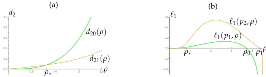
`₁(p₀,c₂₀(ρ),ρ) = (64ρ²+9)(30074175488ρ⁸+9866010240ρ⁶−2504091294ρ⁴−1131103197ρ²−80677701)

169ρ³(4096ρ²+1521)(16384ρ²+1521)(100ρ⁴+1252ρ²+81) . Corollary 2.6. There exists a unique real numberρ₀>0such that`₁(p₀,c₂₀(ρ₀),ρ₀) =0.

Proof. By Lemma2.5,`₁(p₀,c₂₀(ρ),ρ) =0 if and only if

30074175488ρ⁸+9866010240ρ⁶−2504091294ρ⁴−1131103197ρ²−80677701=0. (2.6) According to the Descartes rule, there is a unique real number ρ₀ > 0 such that

`₁(p0,c20(ρ0),ρ0) = 0. Indeed, solving numerically equation (2.6) for the parameter ρ, we have thatρ₀(≈0.57721).

Since `₁(p0,c20(ρ),ρ)takes positive and negative values, we will verify the transversality conditions to have Andronov–Hopf or Bautin bifurcation. At first we state the following result proposed as an exercise in Ref. [6], whose proof is straight forward and we omit the details.

Lemma 2.7. Let M(τ) be a parameter-dependent real (n×n)-matrix which has a simple pair of complex eigenvaluesξ(τ)±iω(τ)such thatξ(τ₀) =0andω(τ₀):= ω₀>0.Then, the derivative of the real part of the complex eigenvalues atτ₀is given by

dξ

dτ(τ0) =Re

p^tr· dM

dτ (τ0)·q

, wherep,q∈_Cⁿare eigenvectors satisfying the normalization conditions

M(τ₀)_q=iω₀, M^tr(τ₀)_p=−iω₀, q^tr·_q=1 and p^tr·_q=1.

We know proceed to show the regularity condition in order to obtain a Bautin bifurcation.

Lemma 2.8(Bautin regularity condition). If the parameters a₁,a2,b2,k2,k3 and d2 satisfy the hy- pothesis of Lemma2.3, then the map(c₂,ρ)7→ (ξ(p₀,c₂,ρ),`₁(p₀,c₂,ρ))is regular at(c₀,ρ₀),where ξ(p₀,c₂,ρ)is given in Remark2.4and c₀ :=c₂₀(ρ₀).

Proof. By hypothesis, the linear approximation of the differential system (2.1) at p₀ depends only on the parametersc₂ andρ, let M_p0(c₂,ρ)be this linear approximation. By Lemma2.5, the complex numbers±₂ⁱ are eigenvalues of Mp₀(c₀,ρ₀), hence, the real part of the complex eigenvalues ofM_p0(c₀,ρ₀), are

ξ(p₀,c₀,ρ₀) =_{0, (2.7)}

letpandqbe eigenvectors ofM_p0(c₀,ρ₀)for the corresponding eigenvalues−₂ⁱ and ₂ⁱ, respec- tively, such that

q^tr·q=1 and p^tr·q=1. (2.8)

By (2.7) and (2.8), we can apply Lemma2.7to the linear approximationMp₀(c₂,ρ), then taking into account the values ofp, q, and ^∂Mp_∂c^0(c2,ρ)

2 , which we compute with the Mathematica soft- ware, we have that the partial derivative of the real part of the eigenvaluesξ(c₂,ρ)±iω(c₂,ρ) of Mp₀(c₂,ρ), with respect to the parameterc₂, at the point(c₀,ρ₀), takes the value

∂ξ

∂c₂(c₀,ρ₀) =p^tr

∂Mp₀(c0,ρ0)

∂c₂ ·q

=− ^1664ρ

20

16384ρ²₀+1521. (2.9) Applying Lemma2.7one more time, and taking into account the values ofp,qand ^∂M(_∂ρ^c2,ρ) it follows that

∂ξ

∂ρ(c₀,ρ₀) =p^tr

∂M_p0(c₀,ρ₀)

∂ρ ·q

= ^{32 38ρ}

20−9

16384ρ²₀+1521. (2.10) From the Kuznetsov formula (see Ref. [4]), the first Lyapunov coefficient at the equilibrium point p₀is given by

`₁(p₀,c₂,ρ) = ^ReC1(c₂,ρ)

ω(c₂,ρ) −ξ(c₂,ρ)^ImC1(c₂,ρ)

ω²(c₂,ρ) ^{, (2.11)} where C₁(c2,ρ) is a function that takes complex values as a differentiable function in the variables(c₂,ρ). Notice that, from Corollary2.6, (2.7), (2.11) and sinceω(c₀,ρ₀) =1/2,

ReC1(c₀,ρ₀) =_{0. (2.12)}

Hence, from (2.11), (2.7) and (2.12), the partial derivative of `₁(c₂,ρ)with respect toc₂ at the point (c₀,ρ₀)is given by

∂`₁

∂c2

(c₀,ρ₀) = ¹ ω²(c0,ρ₀)

ω(c₀,ρ₀)Re ∂C₁

∂c2

(c₀,ρ₀)

−ImC1(c₀,ρ₀)^∂ξ

∂c2

(c₀,ρ₀)

and the partial derivative of`₁(_c2,ρ)with respect to ρat the point(_c0,ρ₀)is given by

∂`₁

∂ρ

(c₀,ρ₀) = ¹ ω²(c₀,ρ₀)

ω(c₀,ρ₀)_Re ∂C1

∂ρ

(c₀,ρ₀)

−ImC1(c₀,ρ₀)^∂ξ

∂ρ

(c₀,ρ₀)

, thus, the determinant of interest reduces to

det

∂ξ

∂c2(c₀,ρ₀) ^∂ξ

∂ρ(c₀,ρ₀)

∂`₁

∂c2(c₀,ρ₀) ^∂`1

∂ρ(c₀,ρ₀)

!

=

∂ξ

∂c2(c0,ρ0)Re

∂C1

∂ρ (c0,ρ0)− ^∂ξ_∂ρ(c0,ρ0)Re

∂C1

∂c2(c0,ρ0)

ω(c₀,ρ₀) ^{. (2.13)}

Numerically, one has that Re ^∂C_∂c¹

2(c₀,ρ₀) ≈ −0.9053 and Re ^∂C_∂ρ¹(c₀,ρ₀) ≈ 2.48325, and by Corollary2.6,ρ₀ ≈0.57721. Then by (2.9), (2.10) and (2.13)

det

∂ξ

∂c2(c₀,ρ₀) ^∂ξ

∂ρ(c₀,ρ₀)

∂`₁

∂c2(c₀,ρ₀) ^∂`1

∂ρ(c₀,ρ₀)

!

≈ −0.18205.

Hence, the map(c₂,ρ)7→(ξ(p₀,c₂,ρ)_,`₁(p₀,c₂,ρ))is regular at(c₀,ρ₀)_.

Theorem 2.9. If the parameters a₁,a₂,b₂,k₂,k₃and d₂satisfy the hypothesis given in Lemma2.3, then the differential system(2.1)exhibits an Andronov–Hopf bifurcation at p₀= √

2,⁵²

√2ρ²

64ρ²+9,^{√ 65ρ4}

2(128ρ²+18)

, with respect to the parameter c2and its bifurcation value is c20(ρ),whereρ>0andρ6=ρ0.Moreover, ifρ >ρ₀the bifurcation is subcritical and ifρ<ρ₀ the bifurcation is supercritical.

Proof. From Lemma 2.3, the linearization Mp₀(c₂,ρ) of differential system (2.1) at p₀ has a positive real eigenvalue and a conjugate pair of pure imaginary eigenvalues if c₂ = c₂₀(ρ). From Lemma2.8, the derivative of the real part of the complex eigenvalues is

∂ξ

∂c2

(c₂₀(ρ),ρ) =− ^1664ρ2 16384ρ²+1521,

which is negative for ρ 6= 0, and hence the transversality condition holds. The Lemma 2.5 and Corollary 2.6 give a negative first Lyapunov coefficient if ρ < ρ₀, and a positive first Lyapunov coefficient ifρ >ρ₀. Then the hypotheses of Andronov–Hopf bifurcation Theorem (see Refs. [7–9]) hold and we conclude the proof.

Lemma 2.10(Second Lyapunov coefficient). If we have the assumptions given in Lemma2.3, then the second Lyapunov coefficient of the differential system(2.1)at the equilibrium point p₀is given by

`₂(p₀,c₂₀(ρ)_,ρ)

=− ^64ρ

2+92

s₁(ρ)

65804544ρ⁹(4096ρ²+1521)³(16384ρ²+1521)³(16384ρ²+13689)s₂(ρ)^{2, (2.14)} where

s₁(ρ) =1684088318371577781870044208361897984ρ²⁶− 12159352425316235727712314958979006464ρ²⁴+ 84451000135751630806296323148790890496ρ²²+ 88370770237252221116361066360845893632ρ²⁰− 109618776714701834747940641433301549056ρ¹⁸− 194370158327281073384907679985062379520ρ¹⁶− 113112389947859122362340150200812175360ρ¹⁴− 33189611310495737671149541682647842816ρ¹²− 5137221528028189621494819571679640576ρ¹⁰− 305998757885518907545964388766063032ρ⁸+ 30440310395959735846728047367564897ρ⁶+ 7031366298566120280440132136776088ρ⁴+ 492932708224495242328372625695584ρ²+ 12343578321586192504727388915456, s2(ρ) =_100ρ⁴+_1252ρ²+_81.

Moreover, ifρ= ρ₀,then`₂(p₀,c₂₀(ρ)_,ρ)6=_0,whereρ₀is given in the Corollary2.6.

Proof. In order to compute the second Lyapunov coefficient`<sub>2</sub>, we apply the Kuznetsov for- mula, (see Ref. [4]). Taking into account the assumptions of this Lemma and using the Math- ematica software, we obtain that the second Lyapunov coefficient `₂(p₀,c₂₀(ρ),ρ), of the dif- ferential system (2.1) at the equilibrium point p₀ is given by (2.14) and `₂(p₀,c₂₀(ρ₀),ρ₀) ≈ 7.40065.

Corollary2.6, Lemma2.8 and Lemma 2.10provide the validity of the necessary and suf- ficient conditions to apply the Bautin bifurcation theorem (see Ref. [4]). In summary we have the following result.

Theorem 2.11(Bautin bifurcation in linear growth). If the parameters a₁,a₂,b₂,k₂,k₃and d₂satisfy the hypothesis given in Lemma 2.3, then the differential system (2.1) exhibits a Bautin bifurcation at p₀,with respect to the parameters c₂andρand its critical bifurcation value is(c₂₀(ρ₀)_,ρ₀)_.

3 Logistic case

In this section we consider the differential system (1.2) with a logistic growth for the prey, this means that the functionh(x) =ρx 1− _R^x and we will analyze the differential system

˙

x=ρx 1− ^x

R

− ^a1xy b₁+x²,

˙

y= ^a1c1xy

b₁+x² − ^a2yz

b₂+y −c₂y, z˙ =z

a2c3y b₂+y −d2

.

(3.1)

In order to make ecological sense we assume that all parameters of the system (3.1) are positive.

Lemma 3.1. If the parameters a₁, a2, b₁, c₁and R, satisfy a₁= ^{ρ b1}+x₀²

(R−x₀)

Ry0 , a₂ = ^d2(b₂+y₀)

c3y0 , R=k₂+x₀, c₁= ^c2c3y0(k₂+x₀) +k₃

c₃k₂ρx₀ , b₁ =k₂x₀+k₄, (3.2)

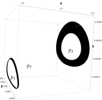
then the unique equilibrium points of the differential system(3.1)in the regionΩare p₁=

x₀,y₀, 2k₃

d₂(k₇+k₈+6x₀)

, p₂=

k₇

2 +x₀,y₀,c₂c₃k₇y₀(k₈+2x₀)(k₇+k₈+6x₀) +2k₃(k₇+2x₀)(k₈+4x₀) 2d₂x₀(k₇+k₈+4x₀)(k₇+k₈+6x₀)

, p₃=

k₈

2 +x₀,y₀,c₂c₃k₈y₀(k₇+2x₀)(k₇+k₈+6x₀) +2k₃(k₇+4x₀)(k₈+2x₀) 2d₂x₀(k₇+k₈+4x₀)(k₇+k₈+6x₀)

. Where, x0 >0, y0 >0, k3 >0, k7≥0, k8≥0and

k₂= ^4x0+k₇+k₈

2 , k₄= ¹

4k₅k₆, k₅=2x₀+k₇, k₆=2x₀+k₈. (3.3)

Proof. The equilibrium points of the differential system (3.1) are the solutions of the system, ρx

1− ^x R

− ^a1xy b1+_x² =0, a₁c₁xy

b₁+x² − ^a2yz

b₂+y −c₂y=0, z

a2c3y b₂+y−d₂

=0.

Multiplying the above equations by b₁+x²

(b₂+y), (which is always positive in the region Ω), we obtain that the equilibrium point must satisfy (3.4). Correspondingly each solution of (3.4) must be an equilibrium point of the differential system (3.1).

a₁Ry−ρ b₁+x²

(R−x) =0, (b₂+y) c₂ b₁+x²

−a₁c₁x

+a₂z b₁+x²

=0, (3.4)

d2(b2+y)−a2c3y=0.

A point(x₀,y₀,z₀)∈_Ωis an equilibrium point of the differential system (3.1) if a₁Ry₀−ρ b₁+x²₀

(R−x₀) =0, (b₂+y₀) c₂ b₁+x²₀

−a₁c₁x₀

+a₂z₀ b₁+x²₀

=0, d₂(b₂+y₀)−a₂c₃y₀=0.

(3.5)

We supposex₀ >_0, y₀ >_{0 and}z₀ >0. Note that the first equation of the system (3.5) is a linear equation in terms ofa₁, and it has the unique solution,

a₁ = ^{ρ b1}+x₀²

(R−x₀)

Ry₀ .

Sincea₁ > 0, R−x₀ must be positive, so there existsk₂ > 0 such thatR = x₀+k₂. A similar argument using the third equation of system (3.5), we obtain that:

a₂= ^d2(b₂+y₀) c₃y₀ .

Using the values of a₁,a₂ and R, and solving the second equation of system (3.5) for z₀, we have that

z₀ = ^c1c3k2ρx0−c₂c₃y₀(k₂+x₀) d₂(k₂+x₀) ^.

Sincez₀> 0, there must existsk₃>0, such thatc₁c₃k₂ρx₀−c₂c₃y₀(k₂+x₀) =k₃. Then c₁= ^c2c3y0(k2+x0) +k3

c₃k₂ρx₀ .

Therefore, if a₁,a₂,R and c₁ satisfy (3.2), then (x₀,y₀,z₀) is a solution of system (3.4) in Ω, wherez₀ = ^k3

d2(k2+x0). Moreover, the system (3.4) takes the form k₂ρy b₁+x₀²

y₀ −ρ b₁+x²

(k₂−x+x₀) =0, (b₂+y) c₂ b₁+x²

−Q

+ ^{d2z b1}+x²

(b₂+y₀)

c₃y₀ =0, (3.6)

b2d2(y0−y) y₀ =0,

where Q= ^x(^b1+x₀²)^(c2c₃y₀(k₂+x₀)+k₃)

c₃x₀y₀(k₂+x₀) . Solving the third equation of system (3.6) for y, we have that y=y₀. Moreover, the first equation of system (3.6) reduce to:

ρ(x−x0) x²−k2x+b₁−k2x0

=0.

Hence, the solutions of this equation are x₀, x₁:= ¹

2

k₂− q

k₂(k₂+4x₀)−4b₁

, x₂:= ¹ 2

k₂+

q

k₂(k₂+4x₀)−4b₁

. Thus, a necessary condition to have at least two solutions of system (3.6) inΩis that k₂(k₂+ 4x₀)−4b₁ ≥ 0. On the other hand, x₁ > 0 if and only if 0 < k²₂−(k₂(k₂+4x₀)−4b₁) = 4(b₁−k₂x₀), then,x₁ >0 if and only if there exists k₄ > 0 such thatb₁ = k₂x₀+k₄, which is a hypothesis in (3.2). Letk₅ =k₂−

q

k₂²−4k₄>0, thenk₄ = ¹₄k₅k₆, wherek₆ =2k₂−k₅>0.

Hence, x₁ = ^k₂⁵ _andx₂ = ^k₂⁶_.

Substituting b₁,k₄,k₅, k₂, y = y₀ and x = x₁ in the second equation of system (3.6) and solving this equation forz, we have that

z₁ = ^c2c3k6y0(k₅−2x₀)(k₅+k₆+2x₀) +2k₃k₅(k₆+2x₀) 2d₂x₀(k₅+k₆)(k₅+k₆+2x₀) ^.

Moreover, if k₅−2x₀ ≥ 0, then z₁ > 0. In the same way, replacingy = y₀ and x = x₂ in (3.6), we obtain

z₂ = ^c2c3k5y0(k₆−2x₀)(k₅+k₆+2x₀) +2k₃k₆(k₅+2x₀) 2d₂x₀(k₅+k₆)(k₅+k₆+2x₀) ^. Also, if k6−2x0 ≥0, thenz2 >0.

Letk₇=k₅−2x₀andk₈=k₆−2x₀, thenx₁ = ^k₂⁷ +x₀,x₂= ^k₂⁸ +x₀, andz₁, z₂ becomes z₁ = ^c2c3k7y0(k8+2x0)(k7+k8+6x0) +2k3(k7+2x0)(k8+4x0)

2d₂x₀(k₇+k₈+4x₀)(k₇+k₈+6x₀) ^, z₂ = ^c2c3k8y0(k₇+2x₀)(k₇+k₈+6x₀) +2k₃(k₇+4x₀)(k₈+2x₀)

2d₂x₀(k₇+k₈+4x₀)(k₇+k₈+6x₀) ^.

Therefore, the unique equilibrium points of the differential system (3.1) in the regionΩ, are:

p₁ = (x₀,y₀,z₀), p₂= (x₁,y₀,z₁) and p₃ = (x₂,y₀,z₂), which completes the proof.

Remark 3.2. Choosing the valuesk₇, k₈adequately, we obtain one, two or three equillibria.

1. Ifk₇= k₈ =0, then p₁= p₂= p₃= x₀,y₀,_3d^k3

2x0

, is the unique equilibrium point of the differential system (3.1) in Ω.

2. Ifk₇=_{0, and}k₈>_{0 then} p₁= p₂= x₀,y₀,_d2k8^2k_+6d³ _2x0 , and p₃ =

k₈

2 +x₀,y₀,c₂c₃k₈y₀(k₈+6x₀) +4k₃(k₈+2x₀) d₂(k₈+4x₀)(k₈+6x₀)

, hence, there are two equilibrium points of the differential system (3.1) in Ω.