Predator–prey systems with small predator’s death rate

Predator–prey systems with small predator’s death rate

Renato Huzak

Hasselt University, Campus Diepenbeek, Agoralaan Gebouw D, 3590 Diepenbeek, Belgium Received 22 April 2018, appeared 9 October 2018

Communicated by Eduardo Liz

Abstract. The goal of our paper is to study canard relaxation oscillations of predator–

prey systems with Holling type II of functional response when the death rate of preda- tor is very small and the conversion rate is uniformly positive. This paper is a natural continuation of [C. Li, H. Zhu, 2013; C. Li, 2016] where both the death rate and the conversion rate are kept very small. We detect all limit periodic sets that can produce the canard relaxation oscillations after perturbations and study their cyclicity by using singular perturbation theory and the family blow-up.

Keywords: predator–prey systems, slow-divergence integral, slow–fast systems.

2010 Mathematics Subject Classification: 34E15, 34E17, 34C26.

1 Introduction

The Rosenzweig–MacArthur predator–prey model is typically given by (x˙ =rx 1− _K^x−y_b^mx_+x

˙

y=y −δ+c_b^mx_+x

, (1.1)

wherex ≥0 is the population density of prey,y≥0 is the population density of predator and all the parameters are strictly positive. The functionP(x) = _b^mx_+xis called the predator response function, δ > 0 represents the death rate of the predator, c > 0 is the rate of conversion of prey to predator and the function x 7→ rx 1− _K^x represents the logistic growth model of the prey in the absence of predator. System (1.1) is a special case of more general predator–prey systems with a Holling type response function P:

(x˙ =_{rx 1}−_K^x−yP(_x)

˙

y=y −δ+cP(x), (1.2)

with the same conditions on x,yand the parameters. The function P in (1.1) is an increasing function and tends to m > _{0 as} x → ∞, and it is often called a Michaelis–Menten function or a response function of Holling type II. We call the function P(x) = _a^mx_+x²₂, with m > 0 and a > 0, the response function of Holling type III, and its generalized version is given

BEmail: renato.huzak@uhasselt.be

by P(x) = _a+^mx_bx+²_x2. The Holling type IV response function or the Monod–Haldane function is given by P(x) = ^mx

a+bx+x², and its simplified version is given by P(x) = ^mx

a+x². For more details about the predator–prey model (1.2) with Holling type of functional responses, see e.g.

[16,18]. We also refer to [9,14,19,20], etc.

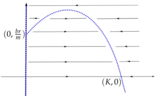
When working with predator–prey system (1.2), we typically assume that the parameters are positive constants kept away from zero. Limit cycles of (1.2), with response functions of Holling type II and generalized Holling types III and IV, have been studied in [15,16], uniformly in (_δ,c) → (_{0, 0})_{. When} δ = c = 0, system (1.2) contains curves of singularities (often called slow curves or critical curves). See e.g. Figure 1.1. Periodic orbits of (1.2) that are Hausdorff close to limit periodic sets, at levelδ = c = 0, containing pieces of the critical curves and fast orbits are called relaxation oscillations (see e.g. [5,6]). Thus, [15,16] deal with the relaxation oscillations of (1.2) when(δ,c)∼ (0, 0), away from the degenerate intersection point 0,^br_m

, using geometric singular perturbation theory [3–5,12].

(K, 0) (0,^br_m)

Figure 1.1: Dynamics of (1.1), withδ =c=0.

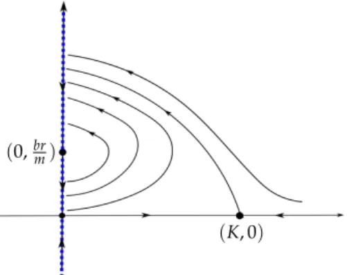
The goal of our paper is to study another limiting case observed in [16]: δ → 0 and cis a positive constant. Whenδ = 0 andc > 0, system (1.2) contains the critical curve {x = 0} (note thatP(0) = 0). Let us focus on system (1.1) (see Figure1.2). All the singularities of the critical curve are normally hyperbolic, except the nilpotent contact point(x,y) = (0,^br_m). We distinguish between 3 types of limit periodic sets, at levelδ=0, that can generate limit cycles whenδ ∼ 0 and δ > 0 (see also Section 2): (i) the nilpotent contact point (x,y) = (0,^br_m), (ii) canard limit cycles consisting of a fast orbit and the part of the critical curve, with a regular slow dynamics, between theα-limit set and theω-limit set of that fast orbit and (iii)the slow–

fast 2-saddle limit periodic set consisting of the hyperbolic saddle (x,y) = (K, 0), the stable manifold of(x,y) = (K, 0), the unstable manifold of(x,y) = (K, 0)and the part of the critical curve between the origin (i.e. theα-limit set of the stable manifold) and theω-limit set of the unstable manifold. (As we will see in Section2, the slow dynamics of (1.1) along the critical curve has a hyperbolic saddle at the origin.)

The goal of our paper is to study the cyclicity of each of these limit periodic sets by using geometric singular perturbation theory and the family blow-up at (x,y,δ) = (0,^br_m, 0). To study the contact point (x,y) = _0,^br_m, we use the theory of slow–fast Hopf points of codimension 1 developed in [12]. To find the cyclicity of the canard limit cycles, we study zeros of the so-called slow-divergence integral of (1.1), using results from [3]. The paper [4]

is a generalization of [3] allowing zeros in the slow dynamics, away from the contact point.

Since the slow–fast 2-saddle limit periodic set contains, beside a zero of the slow dynamics at the origin(x,y) = (0, 0), a (hyperbolic) saddle at (x,y) = (K, 0), away from the critical curve, we cannot use the results of [4] directly. Thus, we have to develop new methods that are suitable for

studying the cyclicity of the slow–fast 2-saddle limit periodic set. Clearly, the new techniques can be used not only in the framework of (1.1) or (1.2), but also in more general planar slow–fast systems.

(K, 0) (0,^br_m)

Figure 1.2: Dynamics of (1.1) forδ=0 andc>0.

In the regular case (δ is a positive constant), the system (1.1) has at most one limit cycle (see [1,13]). The reason we study limit cycles of (1.1) uniformly in δ →0 is twofold. On one hand, we cannot apply the methods of [1,13] to the singular caseδ → 0, and we need to use techniques coming from singular perturbation theory, including the family blow-up. On the other hand, our paper provides a good starting point to get familiar with the methods that can be used not only to study the singular Holling type II case (1.1) but also the more general system (1.2), with a response function of Holling type III and IV, in the singular caseδ →0.

In Section 2 we state our main results. Our upper bounds on the number of limit cycles in (1.1), withδ→0, are 1 or 2, depending on the region in the parameter space (see Theorem 2.2–Theorem2.4). We prove our main results in Section3.

2 Statement of results

We state our main results in Section 2.3–Section 2.5, clearly distinguishing between three different types of limit periodic sets defined in Section 2.2. Instead of working with the original predator–prey model (1.1), it is more convenient to work with a polynomial normal form (2.4) obtained in Section2.1.

2.1 Normal form of (1.1)

Let us recall that r > 0, K > 0, m > 0, b > 0, c > 0 and δ ≥ 0 is the singular perturbation parameter in (1.1). After the rescaling (x, ¯¯ y, ¯b, ¯c, ¯δ) = _K^x,_rK^my,_K^b,^cm_r ,^δ_r

, we may assume that (1.1) has the following form:

(x˙ =x 1−x

− _b^xy_+x

˙

y= y −δ+c_b+^x_x

, (2.1)

where we denote (x, ¯¯ y, ¯b, ¯c, ¯δ)again by (x,y,b,c,δ). Thus, we have that x ≥ 0, y ≥ 0, b > 0, c > _{0 and} δ ≥ 0 is the singular perturbation parameter (δ ∼ 0). Using a time rescaling, i.e.

multiplication byb+x>0, system (2.1) becomes a polynomial vector field:

(x˙ = x b+ (1−b)x−x²−y y˙ =y −δ(b+x) +cx

. (2.2)

Whenδ=0, (2.2) becomes

(x˙ = x b+ (1−b)x−x²−y

˙

y=cxy, (2.3)

and we call (2.3) the fast subsystem of (2.2). The critical curve {x = ₀}of (2.3) is normally attracting wheny > band normally repelling when 0 ≤ y < b. When y = b, we deal with a nilpotent contact point (see Figure1.2). One of the reasons we work with the polynomial system (2.2), instead of (2.1), is that we want to apply a family blow-up of (2.2) to the point (x,y,δ) = (0,b, 0)(see Section2.2). After translation ¯y = y−b, we may also assume that the nilpotent contact point is situated at(x,y) = (0, 0). We get

(x˙ = x (1−b)x−x²−y y˙ = (y+b) −δ(b+x) +cx

, (2.4)

wherex≥0 andy≥ −b(we denote ¯yagain byy).

2.2 Family blow-up at(x,y,δ) = (0, 0, 0) and the slow dynamics along the critical curve

In this section we show that our slow–fast model (2.4), along the critical curve{x=0}, fits into a general framework of [4]. First, let us focus on the dynamics of (2.4), withδ ∼ 0 andδ> 0, along the critical curve but away from the contact point. Center manifolds of(2.4) +0_∂δ^∂, near the critical curve {x = 0}, with y 6= 0, are given by x = O(δ^m), for all m ≥ 1 (this can be easily seen by using asymptotic expansions of center manifolds inδ). After substituting these manifolds forx in the y-component of (2.4), we obtain the dynamics along the critical curve:

˙

y=δ(−b(y+b) +O(δ)). We get theslow dynamicsof (2.4) after dividing this byδ and letting δtend to 0:

y⁰ = −b(y+b), y6=0. (2.5)

Since b> 0, the slow dynamics(2.5) is regular with one (isolated) hyperbolic saddle at y= −b, and this singularity does not coincide with the contact point at y = 0. Thus, when y ≥ −b, the slow dynamics points downwards (see also Figure1.2).

To study the passage from the attracting part {y > 0} to the repelling part {y < 0} of the critical curve, we write δ = δ^˜2, with ˜δ ∼ 0 and ˜δ ≥ 0, and blow up the origin in the (x,y, ˜δ)-space by using the following blow-up formula:

(x,y, ˜δ) = (e²x,¯ ey,¯ eδ¯), e≥0, e∼0, δ¯≥0, (x, ¯¯ y, ¯δ)∈_S². (2.6) To study the blown up vector field in a small neighborhood of the blow-up locus {e = 0}, we use different charts. In the family directional chart{δ^¯=1}, system (2.4), after division by e>0, becomes:

(x˙¯=x¯ (₁−b)ex¯−e³x¯²−y¯

˙¯

y= (ey¯+b) −(b+e²x¯) +cx¯

. (2.7)

When e=0, system (2.7) has the following form:

(x˙¯= −x¯y¯

˙¯

y=−b²+bcx.¯ (2.8)

Clearly, system (2.8) has a center at (x, ¯¯ y) = ^b_c, 0

. After dividing (2.8) by ¯x 6= 0 it can be easily seen that the function H(x, ¯¯ y) = ^y¯₂² −b²ln|x¯|+bcx¯ is a first integral of (2.8). In the phase directional chart {y¯ =1}, system (2.4) can be written as











˙¯

x =x¯ (1−b)ex¯−e³x¯²−1

−2 ¯x(e+b) −δ^¯2(b+e²x¯) +cx¯

˙

e=e(e+b) −δ^¯2(b+e²x¯) +cx¯ δ˙¯=−δ^¯(e+b) −δ^¯2(b+e²x¯) +cx¯

,

(2.9)

after division by e. When e = δ^¯ = 0, (2.9) has two singularities: ¯x = −_2bc¹ _{and ¯}x = _0.

At (x,¯ e, ¯δ) = (−_2bc¹ , 0, 0), (2.9) has a hyperbolic saddle with eigenvalues (1,−¹₂,¹₂), and at (x,¯ e, ¯δ) = (0, 0, 0), we deal with a semi-hyperbolic singularity (the eigenvalues of the linear part are given by (−1, 0, 0)), with a two-dimensional center manifold and with the ¯x-axis as stable manifold. Each center manifold contains the line of singularities{x¯ = δ^¯ = 0}and has the following form: ¯x = O(δ^¯m), for all m ≥ 1. Putting this in the(e, ¯δ)-component of (2.9) we get the following center behavior: {e˙ = eδ¯²(−b²+_O(_{e, ¯}δ))_{, ˙¯}δ = δ^¯3(_b²+_O(_{e, ¯}δ))}, which has, after division byδ¯², an isolated hyperbolic saddle at(e, ¯δ) = (0, 0).

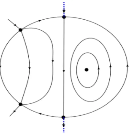
If we apply the coordinate change (e, ¯δ,t) → (−e,−δ,^¯ −t) to (2.9), then we obtain the blown-up vector field in the phase directional chart{y¯=−1}(see (2.6)). In the charts{x¯=1} and{x¯= −1}, we find no extra singularities. See Figure2.1.

Figure 2.1: Dynamics on the blow-up locus of (2.6).

Thus, the passage along the critical curve{x=0}, with y≥ −b, satisfies the assumptions of [4]. Now we define the canard limit cycle Γ⁽y^b,c), y ∈]−b, 0[, consisting of a regular orbit of the fast subsystem of (2.4) and the part of the critical curve between the α-limit set (0,y) and theω-limit set(0,F(y))of that regular orbit, where thefast relation function Fdepends on (b,c)andF(y)>0. Since the slow dynamics (2.5) is regular on the segment[y,F(y)]for each y ∈]−b, 0[, we can use the so-called slow divergence integral of (2.4) along [y,F(y)] to study limit cycles of (2.4) Hausdorff close to Γ⁽y^b,c) (see [3] or [4]). The slow divergence integral is defined as:

I(_y,b,c)_:=

Z _F(y)

y

sds

−b(s+b)^{, y}∈]−b, 0[_{, (2.10)}

where we use the fact that−y is the divergence of (2.4), with δ = 0, along the critical curve {x = ₀} _and dτ = ₋ ^dy

b(y+b) (see (2.5)). Following [3] or [4], the cyclicity of Γ⁽y^b₀^0,c0), with y₀ ∈]−b₀, 0[, near b = b₀ > 0 and c = c₀ > 0, is bounded by the multiplicity of zero of I(y,b0,c0)aty=y0, increased by one.

We denote by Γ⁽₋^b,c_b⁾ the slow–fast 2-saddle limit periodic set in (2.4), at level δ = _{0, con-} sisting of the horizontal orbit y = −b connecting the hyperbolic saddle (x,y) = (0,−b) of the slow dynamics with the hyperbolic saddle (x,y) = (1,−b), the unstable manifold of (x,y) = (1,−b), theω-limit set (x,y) = (0,F(−b)) of the unstable manifold and the critical curve [−b,F(−b)]. Note that Γ⁽y^b,c) → _Γ⁽₋^b,c_b⁾ in the Hausdorff sense as y → −b. Since the segment [−b,F(−b)] contains the singularity of the slow dynamics, we cannot use (2.10) to study the cyclicity ofΓ⁽₋^b,c_b⁾(see [4]). See Sections2.3and3.1for more details.

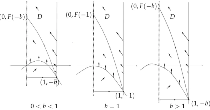
Remark 2.1. Let us explain why the slow–fast 2-saddle limit periodic setΓ⁽₋^b,c_b⁾is well defined for eachb > _{0 and} c > 0, i.e. let us show that F(−b) < _{∞ for all} b > _{0 and} c > _{0. Notice} that the unstable manifold of the hyperbolic saddle (x,y) = (1,−b) in (2.4) with δ = 0 is given byx =1−_b+^y+_c+^b₁ +O((y+b)²). Since the vector field (2.4), with δ =0, points inwards the (positively invariant) set D := {0 ≤ x ≤ 1,y ≥ −b} along the line {x = 1,y > −b}, the unstable manifold enters the set D and stays in D. For the system (2.4), with δ = 0, the parabola y = (1−b)x−x² and the critical curve x = 0 represent the x-nullcline (see Figure2.2). To show thatF(−b) < _∞ for b> 0, we have to study (2.4) near y = +_∞. After a coordinate change(x,y) = (X,_Y¹), withY ∼ 0 andY > 0, and multiplication byY, system (2.4), forδ=0, becomes

(X˙ =X (1−b)XY−X²Y−1

Y˙ =−cXY²(1+Yb). (2.11)

whereX ≥0 andY ≥0. Singularities of (2.11) are given by{X =0}; all the singularities are semi-hyperbolic and attracting. Notice also that{Y=₀}is the stable manifold of the singular point(X,Y) = (0, 0)and that the (local) stable manifold of the singular point(X,Y) = (0,Y₀), with Y₀ ≥ 0 and Y₀ ∼ 0, is the graph of the unique solution of the initial value problem {_dX^dY = ₍ ^−cY2(1+Yb)

1−b)XY−X²Y−1, Y(0) = Y₀}. Since the stable manifolds are unique, we have that F(−b)<_∞.

(1,−1)

(_1,−b) (1,−b)

0<b<₁ b=₁ b>₁

D D D

(0,F(−b)) (0,F(−1))

(0,F(−b))

Figure 2.2: Nullclines and direction field for (2.4) with δ=0.

2.3 Cyclicity ofΓ⁽₋^b,c_b⁾

As explained in Section1and Section2.2, the limit periodic setΓ⁽₋^b,c_b⁾ contains one “singular”

hyperbolic saddle and one “regular” hyperbolic saddle. Using [4,17] and the fact that the connection between the two saddles is unbroken, we show that the singular hyperbolic saddle is dominant, and we obtain the following cyclicity result:

Theorem 2.2. Let b0 >0and c0>0. There exist a smallδ0>0, a neighborhoodW of(b0,c0)in the (b,c)-space and a (Hausdorff) neighborhood V of Γ⁽₋^b_b^0,c₀⁰⁾ such that system(2.4) has at most one limit cycle inV, for each value(δ,b,c)∈[0,δ₀]× W. If the limit cycle exists, it is hyperbolic and repelling.

Theorem2.2 will be proved in Section3.1.

2.4 Cyclicity ofΓ⁽y^b,c)

To study zeros of the slow divergence integral (2.10), first we have to find properties of the fast relation function Fon ]−b, 0[by using a first integral of (2.4), with δ = 0. Whenc= 2b+2, we find the first integral by using Darboux theory of integrability, and we get the following cyclicity result:

Theorem 2.3. Let b₀ > 0, c₀ = 2b₀+2. Suppose that C ⊂]−b₀, 0[ is compact. The following statements are true.

1. If 0 < b₀ < 1, then there exist δ₀ > 0, a neighborhood W of (b₀,c₀)in the (b,c)-space such that the set∪_y∈CΓ⁽_y^b0,c0)can produce at most two limit cycles in (2.4), for each value (δ,b,c)∈ [_0,δ₀]× W.

2. If b₀≥ 1, then there existδ₀ >0, a neighborhoodW of(b₀,c₀)in the (b,c)-space such that the set∪_y∈CΓ⁽_y^b0,c0)can produce at most one limit cycle in(2.4), for each value(δ,b,c)∈[0,δ₀]× W. If the limit cycle exists, then it is hyperbolic and repelling.

Theorem2.3will be proved in Section3.2. The casec6=2b+2 is a topic of further studies.

2.5 Cyclicity of the contact point

To study the number of limit cycles close to a contact point, we typically blow up the contact point and detect all possible limit periodic sets on the blow-up locus that can produce limit cycles after perturbation: a center, closed orbits surrounding the center and a singular cycle consisting of two semi-hyperbolic singularities on the equator of the blow-up locus and the regular orbits that are heteroclinic to them (see Figure 2.1). When b 6= 1, we can bring our system (2.4), near the contact point at the origin, to a normal form for a slow–fast Hopf point of codimension 1 studied in e.g. [12], and we obtain at most one (hyperbolic) limit cycle.

Theorem 2.4. Let b₀>0and c₀>0. The following statements are true:

1. If 0 < b0 < 1, then there exist δ0 > 0, a neighborhood W of (b0,c0)in the (b,c)-space and a neighborhood V of(x,y) = (0, 0)such that system (2.4) has a repelling hyperbolic focus in V and at most one (hyperbolically attracting) limit cycle inV, for each value(δ,b,c)∈]0,δ₀]× W. 2. If b₀ > 1, then there exist δ₀ > 0, a neighborhood W of (b₀,c₀) in the (b,c)-space and a neighborhoodV of(x,y) = (0, 0)such that system(2.4)has an attracting hyperbolic focus inV and at most one (hyperbolically repelling) limit cycle inV, for each value(_δ,b,c)∈]_0,δ₀]× W.

Theorem2.4will be proved in Section3.3.

To study the degenerate case b = 1, we have to deal with higher order Melnikov theory near the center and closed orbits on the blow-up locus, on one hand, and with the so-called birth of canards near the singular cycle (see e.g. [7]), on the other. This is the topic of further studies.

3 Proofs of Theorem 2.2–Theorem 2.4

3.1 Proof of Theorem2.2

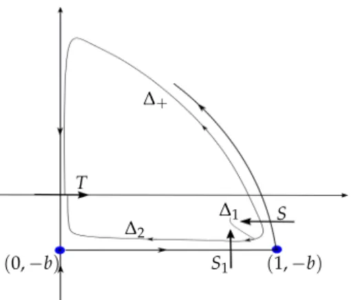
Letb₀ >0 and c₀ > 0 be arbitrary positive constants, and(b,c)∼ (b₀,c₀). System (2.4) has a hyperbolic saddle at(x,y) = (0,−b)with a ratio of eigenvalues−δ^˜2, for each ˜δ>0 and ˜δ ∼0 (δ =δ^˜2). This hyperbolic saddle originates from the hyperbolic singularityy= −bin the slow dynamics (2.5). We also deal with a hyperbolic saddle at(x,y) = (1,−b), for all ˜δ > 0 and δ˜∼0, with eigenvalues ρ₁ =−(1+b)<0 andρ₂ =c−δ^˜2(b+1)>0. Note that the connection between the two saddles is unbroken, i.e. the orbit inside {y = −b}connects (x,y) = (0,−b)and (x,y) = (1,−b), for allδ˜>0,δ˜∼0and(b,c)∼ (b₀,c₀). See Figure3.1.

We define a difference map near the slow–fast 2-saddle limit periodic setΓ⁽₋^b_b^0,c₀⁰⁾:

∆(x, ˜δ,b,c):=_∆+(x, ˜δ,b,c)−_∆−(x, ˜δ,b,c), (δ,^˜ b,c)∼ (0,b0,c0),

where ∆+ (resp. ∆−) is a transition map of (2.4) in forward time (resp. in backward time) fromSto T (see Figure3.1). The horizontal sectionSis parametrized by x(we give a precise definition of S later in this section) and the section T ⊂ {y¯ = 0} is defined in the family directional chart of (2.6) and parametrized by ¯x ∼0, where(x, ¯¯ y)are the coordinates of (2.7).

Thus,T is transverse to the connection{x¯ =0}, on the blow-up locus, between the attracting part of the critical curve and the repelling part of the critical curve (see Figure 2.1). It is clear that limit cycles of (2.4), close to Γ⁽₋^b_b^0,c₀⁰⁾in the Hausdorff sense, are given as zeros of the difference map ∆. In the rest of this section, we show that ∆ has at most one zero in x (counting multiplicity), for each fixedδ˜>0,δ˜∼0and(b,c)∼ (b₀,c₀).

(0,−b) (1,−b)

T

S S₁

∆1

∆2

∆+

Figure 3.1: Limit cycles of (2.4), Hausdorff close to Γ⁽₋^b,c_b⁾, can be studied as zeros of a difference map ∆ := _∆+−_∆− where ∆+ (resp. ∆− = _∆2◦_∆1) is a transition map defined by following the trajectories of (2.4) in forward time (resp. in backward time) from the sectionSto the sectionT.

First, we study the transition map∆−. We split up∆− into two parts (see Figure3.1):

1. The Dulac map∆1 near the hyperbolic saddle (x,y) = (1,−b)defined by following the orbits of (2.4) in backward time fromStoS₁. We study the transition∆1by using results from e.g. [17].

2. The transition map ∆2 defined by following the trajectories of (2.4) in backward time from S₁ to T. This transition map includes the passage near the critical curve with a hyperbolic saddle in the slow dynamics and it has been studied in detail in [4] or [11].

The Dulac map ∆1, near the hyperbolic saddle (1,−b₀), has the following form in the C^k- normal form coordinates (see e.g. [2,17]):

∆1(x, ˜δ,b,c) =x^ρ(1+_Ψ(x, ˜δ,b,c)), (3.1) where x ∼ 0, x > 0, ρ = −^ρ_ρ²

1 = ₁₊^c_b −δ^˜2 > 0, Ψ is a C^∞-function for x > 0 and (δ,^˜ b,c) ∼ (0,b₀,c₀)and

∀n∈_N0: lim

x→0xⁿ∂ⁿΨ

∂xⁿ =0, uniformly in(δ,^˜ b,c)∼(0,b₀,c₀). (3.2) In the normal form coordinates, which we denote again by (x,y), the hyperbolic saddle cor- responds to the origin(x,y) = (0, 0),S⊂ {y=1}is parametrized byx∼0 andS₁ ⊂ {x=1} is parametrized by y∼0. Using (3.1) and (3.2), we obtain:

∂∆1

∂x (x, ˜δ,b,c) =x^ρ−1(ρ+_Φ(x, ˜δ,b,c)), (3.3) where Φ has the property (3.2). On the other hand, the derivative of the transition map ∆2

has the following form (see [4] or [11, Section 3.8.5]):

∂∆2

∂y (y, ˜δ,b,c) = ¹ δ˜⁴exp 1

δ˜² Z ₁

α(y, ˜δ,b,c)

−₁+δ^˜2

s ds+O(₁)

= ¹ δ˜⁴

exp 1 δ˜²

(1−δ^˜2)lnα(y, ˜δ,b,c) +O(1), (3.4) where the section S₁ is parametrized by the above normal form coordinate y ∼ 0, αis aC^k- function in (y, ˜δ,b,c) ∼ (0, 0,b0,c0), with ^∂α_∂y > 0, and theO(1)-term in (3.4) is ˜δ-regularlyC^k in(y,b,c), i.e.O(1)and all its derivatives up to orderkw.r.t.(y,b,c)are continuous including at ˜δ = 0. The integral in (3.4) is the divergence integral of (2.4) near the hyperbolic saddle (0,−b0), multiplied by ˜δ²and calculated inC^k-normal form coordinates{v˙₁ =δ^˜2v₁, ˙v2 =−v2} from {v₂ = 1}, parametrized by v₁ ∼ 0, to{v₁ = 1}, parametrized by v₂ ∼ 0. We supposed that the orbit starting at a point on the sectionS₁, parametrized byy∼0, intersects the section {v2=1}in a point withv₁ =α(y, ˜δ,b,c). Since the connection between(0,−b)and(1,−b)is unbroken, we can write α=yα, where ˜˜ α>0.

Using (3.3) and (3.4), the derivative of∆−w.r.t.x can be written as:

∂∆−

∂x (x) = ^∂∆2

∂y (_∆1(x))^∂∆1

∂x (x)

= ¹ δ˜⁴exp 1

δ˜²

(₁−δ^˜2)_lnα(_∆1(x)) +δ^˜2(ρ−1)_lnx+O(₁) +δ^˜2ln(ρ+_Φ(x)) _(3.5) where, for the sake of readability, we write xinstead of (x, ˜δ,b,c)_andy instead of (y, ˜δ,b,c)_. Note that the term O(1) +δ^˜2ln(ρ+_Φ(x)) in (3.5) is bounded. Sinceα = yα˜ and ˜α >0, (3.1) implies that:

α(_∆1(x)) =x^ρ(₁+_Ψ(x))α˜(_∆1(x))_,

where(1+_Ψ(x))α˜(_∆1(x))is strictly positive and bounded. Thus, (3.5) has the following form:

∂∆−

∂x (x) = ¹ δ˜⁴exp 1

δ˜²

(ρ−δ^˜2)lnx+O−(1) (3.6) for a bounded functionO−(1).

Since the slow dynamics (2.5) is regular fory ≥0, we use e.g. [3] to find the derivative of

∆+ w.r.t.x:

∂∆+

∂x (x) = ¹ δ˜⁴

exp 1 δ˜²

O+(1) (3.7)

whereO+(₁)_{is ˜}δ-regularlyC^kin(_x,b,c), thus bounded. Let us introduce the analytic function E(β₁,β2) = ^expβ_β^1−expβ2

1−β₂ > 0, β₁ 6= β2, and E(β₁,β₁) = expβ₁. Combining (3.6) and (3.7) we get the expression for the derivative of the difference map:

∂∆

∂x(x) = ^∂(_∆+−_∆−)

∂x (x)

= ¹ δ˜⁶

E(β₁,β₂)−(ρ−δ^˜2)lnx+O(1) (3.8) whereO(₁)is a bounded function, β₁ = ¹_˜

δ²O+(₁)_andβ₂ = ¹_˜

δ² (ρ−δ^˜2)_lnx+O−(₁)_{. It thus} suffices to study zeros of the function

−(ρ−δ^˜2)_lnx+O(₁) _(3.9)

introduced in (3.8). Since −(ρ−δ^˜2)lnx → +_∞ as x → 0, (3.9) is strictly positive forx > 0, x ∼_{0 and}(_δ,^˜ b,c)∼(_0,b₀,c₀). Rolle’s theorem implies that the difference map∆has at most one zero (counting multiplicity) w.r.t. x ∼0, x > 0, i.e. Γ⁽₋^b_b^0,c₀⁰⁾can produce at most one limit cycle. It the limit cycle exists, it is hyperbolic and repelling because (3.9) is strictly positive.

This completes the proof of Theorem2.2.

3.2 Proof of Theorem2.3

Let b₀ be an arbitrary positive constant and c₀ = 2b₀+2. We suppose that C ⊂]−b₀, 0[ is an arbitrary compact set. We study zeros of the slow divergence integralI(y,b₀,c₀), given in (2.10), w.r.t.y∈C, depending on the constantb0.

When (δ,b,c) = (0,b₀,c₀), using Darboux theory of integrability, we find the first in- tegral of (2.4), divided by x (i.e. the first integral of the system {x˙ = (1−b0)x−x²−y,

˙

y=c₀(y+b₀)}):

H(x,y) = (2b₀+2)arctan x+b₀

py+b₀ +2p

y+b₀, y>−b₀.

SinceH(0,y) =H(0,F(y))for ally∈]−b₀, 0[, withFintroduced in (2.10), it can be easily seen thatF is analytic on]−b0, 0]and that the derivative ofFhas the following form:

F⁰(y) = ^h(y)

h(F(y))^{, y}∈]−b₀, 0[, (3.10)

where h(y) = √ ^y

y+b0(b²₀+b0+y). Using (2.10) and (3.10), the derivative of the slow divergence integral w.r.t. ycan be written as:

∂I

∂y(y,b₀,c₀)

= −¹ b₀

F(y)F⁰(y) F(y) +b₀ − ^y

y+b₀

= ^h(y) b₀p

F(y) +b₀p y+b₀

q

F(y) +b0(b²₀+b0+y)−^py+b0(b²₀+b0+F(y))

. (3.11) From (3.11) it follows that_∂I

∂y =0 is equivalent to {L(y) =0}, on]−b₀, 0[, where L(y) =

q

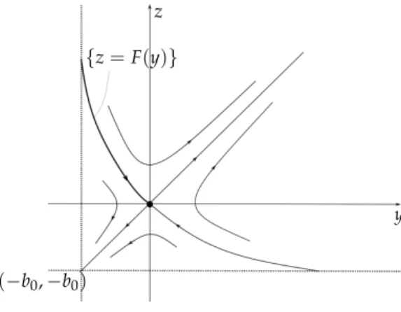
F(y) +b₀(b²₀+b₀+y)−^py+b₀(b²₀+b₀+F(y)). (3.12) On the other hand, (3.10) implies that{z = _F(_y)}is an orbit of the system{y˙ =_h(_z)_{, ˙z} = h(y)}, wherey,z>−b₀. Multiplying this system byp

y+b₀(b²₀+b₀+y)√

z+b₀(b₀²+b₀+z)

>0 yields:

(y˙= zp

y+b₀(b²₀+b₀+y)

˙ z =y√

z+b₀(b²₀+b₀+z), (3.13) where y,z > −b₀. System (3.13) has a hyperbolic saddle at the origin (y,z) = (_{0, 0}) _(see Figure3.2).

(−b₀,−b₀)

y z

{z=F(y)}

Figure 3.2: Dynamics of system (3.13).

In the rest of this section, we show that there exists at most one intersection (counting multiplicity) between{z= F(y)}and{L(y,z) =0}in the region{−b0< y<0,z >0}where the functionLis given by

L(y,z) =^pz+b₀(b₀²+b₀+y)−^py+b₀(b²₀+b₀+z). (3.14) (We replace F(y) by z in (3.12).) This will imply that _∂y^∂I has at most one zero (counting multiplicity) on ]−b₀, 0[. It can be easily seen that each solution of {L(y,z) = ₀} _satisfies y=zor

z =b₀b₀(b²₀−1)−y

y+b0 . (3.15)

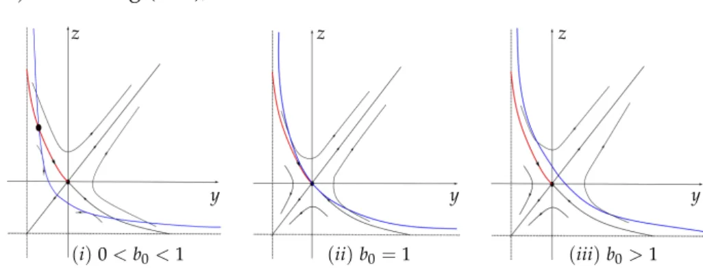
When 0 < b₀ < 1 (resp. b₀ ≥ 1), we prove that there is one transversal intersection (resp.

there are no intersections) between the curve {z = F(y)} and the curve given by (3.15), in

{−b₀ < y < 0,z > 0}(see Figure 3.3). To prove it, first we calculate the number of contact points between the curve{L(y,z) =0}and the orbits of system (3.13). The contact points are given by:

∇L(y,z)· zp

y+b₀(b²₀+b₀+y),yp

z+b₀(b²₀+b₀+z)=0 (3.16) whereL(y,z) =0. Using (3.14), we have that

(i)0<b₀<1 (ii)b₀=1 (iii)b₀>1 y

z

y z

y z

Figure 3.3: When 0 < b₀ < 1, there exist one transversal intersection between {z= F(y)}and{L(y,z) =0}in the region{−b0 <y<0,z >0}. Whenb0 ≥1, there are no intersections in{−b₀ <y<0,z >0}.

∇L(y,z) = ^pz+b₀−¹ 2

b²₀+b0+z

py+b₀ ,−^py+b₀+ ¹ 2

b²₀+b0+y

√z+b₀

! , and (3.16) becomes

(y−z) 1

2(b²₀+b₀+y)(b²₀+b₀+z)−(b²₀+b₀)^py+b₀p z+b₀

=0.

We focus on 1

2(b₀²+b0+y)(b₀²+b0+z)−(b₀²+b0)^py+b0

pz+b0=0. (3.17) WhenL(y,z) =0, then (3.17) is equivalent to

y²+b²₀(b²₀−1) =0.

We distinguish between two cases:

1. When 0< b₀ <1, we have the following contact points between the curve{L(y,z) =0} and the orbits of (3.13): P₁ = −b₀√

1−b²₀,b₀√

1−b²₀

, P₂ = b₀√

1−b²₀,−b₀√ 1−b²₀ and the liney=z. Sincezin (3.15) tends to+_∞asy→ −b₀, there exists at least one in- tersection point between{z=F(y)}and{L(y,z) =0}in the region{−b₀<y<0,z>0} (see Figure3.3(i)). If we suppose that there are at least 2 intersection points (counting multiplicity) between {z = F(y)} and {L(y,z) = 0} in {−b0 < y < 0,z > 0}, then there are at least 2 contact points in{−b₀ <y <0,z >0}. This is in clear contradiction with the fact that there is only one contact point (P₁) in {−b₀ < y < 0,z > 0}. Thus, there exists one transversal intersection point between {z = F(y)} and {L(y,z) = 0} in {−b₀ < y < 0,z > 0}. This implies that ^∂I_∂y has one simple zero on]−b₀, 0[. Using Rolle’s theorem and the fact thatI(0,b₀,c₀) =0, we have that I(y,b₀,c₀)has at most one simple zero on]−b₀, 0[. Thus, at most two limit cycles can be created.

2. When b₀ ≥ 1, the contact points are given by y = z. Suppose there is at least one intersection point between{z= F(y)}and{L(y,z) =0}in {−b0< y<0,z>0}. Then there exists at least one contact point between the curve{L(y,z) =0}and the orbits of system (3.13) in{−b₀ < y < 0,z > 0}, which is a contradiction and proves that there are no intersection points. See Figure 3.3(ii)–(iii). This implies that _∂y^∂I(y,b0,c0) has no zeros on]−b₀, 0[. Using Rolle’s theorem and I(0,b₀,c₀) =0, we have that I(y,b₀,c₀)is strictly positive on]−b₀, 0[. Thus, at most one (hyperbolic and repelling) limit cycle can be created.

3.3 Proof of Theorem2.4

Let b₀ > 0, b₀ 6= 1 and c₀ > 0. We bring (2.4), near the origin (x,y) = (0, 0), withδ = δ^˜2, to a normal form for a slow–fast Hopf point of codimension 1 studied in e.g. [12]. (We suppose that(δ,^˜ b,c)∼ (0,b0,c0).) The change of coordinates ¯x=−δ^˜2b+ (c−δ^˜2)x, with(x,y)∼ (0, 0), changes (2.4) to

(x˙¯= (α₀−y)x¯+δ^˜2(δβ^˜ ₀−by) +γ₀x¯²− ¹

(c−δ^˜2)²x¯³

y˙= (_y+_b)x,¯ (3.18)

where

α₀ =2 ˜δ²b1−b c−δ^˜2

− ^{3 ˜δ}

4b²

(c−δ^˜2)^{2, β0}=δb^{˜ 2}1−b c−δ^˜2

− ^δ˜

3b³

(c−δ^˜2)^{2, γ0}= ¹−b c−δ^˜2

− ^{3 ˜δ}

2b (c−δ^˜2)^2. After the coordinate change X= (y+b)x, for¯ (x,¯ y)∼(0, 0), (3.18) becomes

(X˙ = (α₀−y)X+δ^˜2 δbβ˜ ₀−(b²−δβ^˜ ₀)y−by²

+¹_y⁺₊^γ_b⁰X²− ₍ ¹

c−δ^˜2)²(y+b)²X³

˙

y= X, (3.19)

whereα₀, β₀andγ₀ are given in (3.18). The translationY=y−α₀ brings (3.19) to











X˙ = −YX+δ^˜2

δbβ˜ ₀−α₀(b²−δβ^˜ ₀)−bα²₀

−(b²−δβ^˜ ₀+2bα₀)Y−bY² +_Y+^1+γ0

α0+bX²− ¹

(c−δ^˜2)²(Y+α0+b)²X³ Y˙ = X.

(3.20)

After rescaling (X,Y) = (b²−δβ^˜ ₀+2bα₀)X,^˜

√

b²−δβ^˜ ₀+2bα₀Y˜

and dividing by a positive function

√

b²−δβ^˜ ₀+_2bα0, (3.20) changes into







X˙˜ =−Y^˜X˜ +δ^˜2

β˜₀−Y^˜ − 1+O(δ^˜2)Y^˜2

+ 1+¹⁻_c^b+O(δ^˜2, ˜X, ˜Y)X^˜2 Y˙˜ = X,^˜

where

β˜₀= ^{δbβ˜ 0}−α₀(b²−δβ^˜ ₀)−bα²₀ (b²−δβ^˜ ₀+2bα₀)³² = δ^˜2

b−₁

c +O(δ^˜2)

=_{: ˜}δβ¯₀. (3.21) If we write (x, ˜˜ y) = (Y, ˜^˜ X), we get:







˙˜

x=y˜

˙˜

y=−x˜y˜+δ^˜2

δ˜β¯₀−x˜− 1+O(δ^˜2)x˜²

+ 1+ ¹⁻_c^b+O(δ^˜2, ˜x, ˜y)y˜², (3.22)

where ¯β₀ = δ^{˜ b−}_c¹ +O(δ^˜2) ∼ 0 is given in (3.21). When 0 < b₀ < 1 (resp. b₀ > 1), it can be easily seen that (3.22) has a repelling hyperbolic focus (resp. an attracting hyperbolic focus) near the origin(x, ˜˜ y) = (0, 0), for each(δ,^˜ b,c)∼(0,b₀,c₀)and ˜δ>0.

We write the O(y˜²)-term in (3.22) as O(y˜²) = y˜²G(x, ˜˜ y, ˜δ,b,c), where G is analytic and G(0, 0, 0,b₀,c₀) =1+¹⁻_c^b0

0 . We denote byX_{(δ,b,c˜ )}the system{x˙˜=1, ˙˜y=−x˜+yG˜ (x, ˜˜ y, ˜δ,b,c)}. Let ˜y=h(x; ˆ˜ y, ˜δ,b,c), with hanalytic andh(0; ˆy, ˜δ,b,c) =y, be the solutions ofˆ

dy˜

dx˜ =−x˜+yG˜ (x, ˜˜ y, ˜δ,b,c). (3.23) Using (3.23), we haveh(0; 0, ˜δ,b,c) = _∂^∂h_x˜(0; 0, ˜δ,b,c) =0, ^∂_∂²_x˜^h2(0; 0, ˜δ,b,c) =−1, _∂^∂3_x˜^h3(0; 0, ˜δ,b,c) =

−G(0, 0, ˜δ,b,c), ^∂h_∂yˆ(0; 0, ˜δ,b,c) =1 and _∂^∂_x∂˜^2h_yˆ(0; 0, ˜δ,b,c) =G(0, 0, ˜δ,b,c). The coordinate change

˜

y = h(x; ˆ˜ y, ˜δ,b,c) brings X_{(δ,b,c˜ )} to the box flow 1_∂^∂_x˜, and consequently the vector field (3.22)

becomes 





˙˜

x =h(x; ˆ˜ y, ˜δ,b,c)_.^∂h

∂yˆ(x; ˆ˜ y, ˜δ,b,c)

˙ˆ y=δ^˜2

δ˜β¯₀−x˜− 1+O(δ^˜2)x˜²

, (3.24)

after multiplication by ^∂h_∂yˆ(x; ˆ˜ y, ˜δ,b,c)>0. Using the properties ofh, (3.24) can be written as







˙˜

x=yhˆ ₁(x, ˆ˜ y, ˜δ,b,c) +x˜²h₂(x, ˆ˜ y, ˜δ,b,c)

˙ˆ y= δ^˜2

δ˜β¯₀−x˜− 1+O(δ^˜2)x˜² ,

withh₁ =1+O(x, ˆ˜ y),h₂= −¹₂+O(x, ˆ˜ y), ^∂h_∂x˜¹(0, 0, ˜δ,b,c) =2G(0, 0, ˜δ,b,c)and^∂h_∂x˜²(0, 0, ˜δ,b,c) =

−²₃G(0, 0, ˜δ,b,c). After rescaling(x, ˆ˜ y) = (2x, 2y)and multiplication by−1, we finally get the desired normal form for the so-called non-degenerate canard point (see (3.3) of [12]):







˙

x= −yH₁(x,y, ˜δ,b,c) +x²H₂(x,y, ˜δ,b,c)

˙ y=δ^˜2

xH₃(x,y, ˜δ,b,c)−λ

, (3.25)

with λ = ^δ˜β₂^¯0, H_k = 1 +O(x,y), k = 1, 2, 3, ^∂H_∂x¹(0, 0, 0,b₀,c₀) = 4G(0, 0, 0,b₀,c₀),

∂H2

∂x (0, 0, 0,b₀,c₀) = ⁸₃G(0, 0, 0,b₀,c₀)and ^∂H_∂x³(0, 0, 0,b₀,c₀) =2. Following [12], the sign of A=−^∂H1

∂x (0, 0, 0,b₀,c₀) +3∂H₂

∂x (0, 0, 0,b₀,c₀)−2∂H₃

∂x (0, 0, 0,b₀,c₀) =41−b₀ c₀

determines the dynamics of (3.25) near the origin(x,y) = (0, 0). When 0< b₀ <1 (i.e.A>0), then (3.25) has at most one (hyperbolically repelling) limit cycle in a fixed neighborhood of (x,y) = (0, 0), for each (δ,^˜ b,c) ∼ (0,b₀,c₀). When the limit cycle exists, it is generated by a subcritical Hopf bifurcation atλ =0, taking λ∼ 0 as independent (breaking) parameter (see Theorem 4.2 of [12]). After changing time, we get Theorem2.4. 1. When b₀ > _{1 (i.e.} A < _0), then (3.25) has at most one (hyperbolically attracting) limit cycle in a fixed neighborhood of (x,y) = (0, 0), for each (δ,^˜ b,c) ∼ (0,b₀,c₀). If the limit cycle exists, it is created by a supercritical Hopf bifurcation atλ=_{0, taking}λ∼0 as independent parameter (see Theorem 4.1 of [12]). After changing time, this implies Theorem2.4. 2.

Remark 3.1. Note that the obtained result (at most one small limit cycle when b₀ 6= 1) is compatible with results of [8,10] applied to the normal form (3.22). In the Liénard plane

( ˜y→y˜−¹₂x˜²), (3.22) becomes







˙˜

x= y˜− ¹₂x˜²

˙˜

y=δ^˜2

δ˜β¯₀−x˜− 1+O(δ^˜2)x˜²

+ 1+ ¹⁻_c^b+O(δ^˜2, ˜x, ˜y−¹₂x˜²)(y˜− ¹₂x˜²)². (3.26) After rescaling (x, ˜˜ y) = (δx, ˜^˜ δ²y), with (x,y) kept in a large compact set, and after division by ˜δ > 0, (3.26) becomes {x˙ = y− ¹₂x², ˙y = β^¯0−x−(1+O(δ^˜2))δx^{˜ 2}+ (1+¹⁻_c^b+O(δ^˜))δ^˜(y−

1

2x²)²}. When ˜δ =0, this system has the center at the origin(x,y) = (0, 0), an integrating fac- tor−e^−yand the functionH(x,y) =e^−y(y−¹₂x²+1)as first integral. The center is represented byL₁:={H(x,y) =1}and we denote the closed level curves ofH byL_h, whereh∈]0, 1[. We writeJ₀(h) =R

L_he^−ydxandJ₁(h) =−R

L_he^−yx²dx+ (1+¹⁻_c^b)R

L_he^−y(y−¹₂x²)²dx, forh ∈]0, 1], where L_h is oriented counter-clockwise. SinceR

L_he^−y(y−¹₂x²)²dx= R

L_he^−yx²dx(see [10]), we have that J₁(h) = ¹⁻_c^bR

L_he^−yx²dx, and based on [8] andb₀6=1, it can be proved (see[10]) that the system{_dh^d J₀,_dh^d J₁}of analytic functions is a strict Chebyshev system on[h₀, 1]of degree 1, for all small h₀>0 and(b,c)∼ (b₀,c₀), i.e. at most one limit cycle can be created.

References

[1] K. S. Cheng, Uniqueness of a limit cycle for a predator–prey system,SIAM J. Math. Anal.

12(1981), No. 4, 541–548.https://doi.org/10.1137/0512047;MR0617713

[2] F. Dumortier, M. El Morsalani, C. Rousseau, Hilbert’s 16th problem for quadratic systems and cyclicity of elementary graphics, Nonlinearity 9(1996), No. 5, 1209–1261.

https://doi.org/10.1088/0951-7715/9/5/008;MR1416474;Zbl 0895.58046

[3] P. De Maesschalck, F. Dumortier, Time analysis and entry-exit relation near planar turning points, J. Differential Equations 215(2005), No. 2, 225–267. https://doi.org/10.

1016/j.jde.2005.01.004;MR2147463;Zbl 1075.34048

[4] P. De Maesschalck, F. Dumortier, Canard cycles in the presence of slow dynamics with singularities, Proc. Roy. Soc. Edinburgh Sect. A 138(2008), No. 2, 265–299. https:

//doi.org/10.1017/S0308210506000199;MR2406691;Zbl 1263.37034

[5] F. Dumortier, R. Roussarie, Canard cycles and center manifolds, Mem. Amer. Math.

Soc. 121(1996), No. 577, x+100 pp. https://doi.org/10.1090/memo/0577; MR1327208;

Zbl 0851.34057

[6] F. Dumortier, R. Roussarie, Canard cycles with two breaking parameters,Discrete Con- tin. Dyn. Syst. 17(2007), No. 4, 787–806. https://doi.org/10.3934/dcds.2007.17.787;

MR2276475

[7] F. Dumortier, R. Roussarie, Birth of canard cycles, Discrete Contin. Dyn. Syst. Ser.

S 2(2009), No. 4, 723–781. https://doi.org/10.3934/dcdss.2009.2.723; MR2552119;

Zbl 1186.34080

[8] J. L. Figueras, W. Tucker, J. Villadelprat, Computer-assisted techniques for the verifi- cation of the Chebyshev property of Abelian integrals,J. Differential Equations254(2013), No. 8, 3647–3663.https://doi.org/10.1016/j.jde.2013.01.036;MR3020891