1 Authors:
Peter Sarcevica, Zoltan Kincsesb, Szilveszter Pletlc Title:
Online human movement classification using wrist-worn wireless sensors
Affiliations:
a Technical Department, Faculty of Engineering, University of Szeged Moszkvai krt. 9, 6725 Szeged, Hungary
b,c Department of Technical Informatics, Faculty of Science and Informatics, University of Szeged Arpad ter 2, 6720 Szeged, Hungary
E-mail address of the corresponding author:
sarcevic@mk.u-szeged.hu
Telephone number of the corresponding author:
+36-62-546-571 ORCID:
a 0000-0003-4050-8231
b 0000-0002-7130-9510
c 0000-0002-8721-6271
Acknowledgments:
The publication is supported by the European Union and co-funded by the European Social Fund. Project title:
"Telemedicine-focused research activities on the field of Mathematics, Informatics and Medical sciences"
Project number: TÁMOP-4.2.2.A-11/1/KONV-2012-0073.
Conflict of Interest: The authors declare that they have no conflict of interest.
This is a post-peer-review, pre-copyedit version of an article published in Journal of Ambient Intelligence and Humanized Computing. The final authenticated version is available online at: http://dx.doi.org/10.1007/s12652-017-0606-1
2
Abstract: The monitoring and analysis of human motion can provide valuable information for various applications. This work gives a comprehensive overview about existing methods, and a prototype system is also presented, capable of detecting different human arm and body movements using wrist-mounted wireless sensors.
The wireless units are equipped with three tri-axial sensors, an accelerometer, a gyroscope, and a magnetometer.
Data acquisition was done for multiple activities with the help of the used prototype system. A new online classification algorithm was developed, which enables easy implementation on the used hardware. To explore the optimal configuration, multiple datasets were tested using different feature extraction approaches, sampling frequencies, processing window widths, and used sensor combinations. The applied datasets were constructed using data collected with the help of multiple subjects. Results show that nearly 100% recognition rate can be achieved on training data, while almost 90% can be reached on validation data, which were not utilized during the training classifiers. This shows high correlation in the movements of different persons, since the training and validation datasets were constructed of data from different subjects.
Keywords: activity recognition, wearable sensors, feature extraction, time-domain analysis, dimension reduction
1 Introduction
The analysis and real-time monitoring of human body motion is a widely-studied field of industrial, entertainment, health, and medical applications (Cornacchia et al. 2017). Such systems can be used for robot control, human-computer interaction, assisted living, gaming, fall detection, epileptic seizure detection, telerehabilitation, analysis of daily activities, emergency detection, health monitoring, or even human worker activity recognition in industrial environments.
Human motion can be split into two basic categories, activities and movements. Movements typically last for several milliseconds or seconds, while an activity comprises of different movements, and can last for even minutes or hours (Varkey et al. 2012). For example, a “walking” activity contains several short physical leg movements. But more complex activities can also be defined, such as “cooking”, which is composed of multiple shorter activities in a specific sequence, like “walking”, “arm raising”, “standing”, etc.
Sensor-based motion recognition integrates the emerging area of sensor networks with machine learning techniques. Inertial and magnetic sensors are widely used in wearable devices for motion recognition, due to their small size, low cost, and small energy consumption. These wearable devices applied to human bodies form Wireless Body Sensor Networks (WBSNs) (Alemdar and Ersoy 2010). Another option for human motion monitoring can be the use of Personal Area Networks (PANs), which are composed of environmental sensors, like Radio-Frequency Identification (RFID) readers, video cameras, or sound, pressure, temperature, luminosity, and humidity sensors. The vision-based activity recognition systems are the most popular types of PANs. One of the main advantages of body sensor networks to systems using cameras with fix places is that they support persistent monitoring of a subject during daily activities both in indoor and outdoor environments. The vision- based systems are also influenced by environmental factors, such as lighting conditions, and they incur a significant amount of computational cost.
Due to the difficult implementation of signal processing algorithms on resource constrained wireless nodes, the design of WBSN-based applications is a very complex task (Aiello et al. 2011; Gravina et al. 2017). Efficient implementation of WBSN applications requires appropriate usage of energy, memory, and processing. These systems must meet computational and storage requirements. They should also be wearable, which affects the possible usable battery size and therefore its duration. This is a challenging task, because these applications usually require high sampling rates of the sensors, real-time data processing, and high transmission capabilities.
The goal of this research was to develop a wearable wireless system which does not disturb the user in free movement, and which can efficiently recognize basic body and arm movements using an online classification algorithm. It was also important to explore different setups to minimize the cost, the energy consumption, and the memory requirements, besides maximizing the classification efficiency.
In the study, a prototype system is proposed which uses 9DoF sensor boards mounted on Wireless Sensor Network (WSN) motes, which were attached to the wrists of the subjects. The developed system was used to record measurements for multiple activities. The proposed system does not require any additional server for the processing of the data, and it is also suitable for the logging of the activities.
Related works (described in Sect. 2) mainly do not deal with the implementability of the algorithms on the used hardware, or use a centralized server to do the necessary computation. The use of processing servers can
3
cause several disadvantages. First, the communication in the network is very costly due to the high sampling frequencies of the sensors, and secondly, since the subjects are moving, they can get out of the range of the server if its place is fixed. Some works implement their algorithm on a smartphone, but the performance of these systems can be affected by the varying placement of the units, or their use during the operation of the algorithm.
Based on the above considerations, it was reasonable to develop an online method, and to examine the hardware implementability of different classification algorithms. Linear discriminant analysis (LDA)-based dimension reduction was also tested to investigate its effect on the tested classification methods in the meaning of recognition efficiency, memory consumption, and training time.
Since related studies mainly consider complex activities or use more than 1-2 seconds of data for classification of motions, it was necessary to investigate the barriers in the performance when decreasing the processing window width. Related works which utilize multiple sensor types also do not consider the effect of different sensor types on classification efficiency. To find the optimal setup, multiple classification methods were investigated for various datasets, which were generated based on different sampling frequencies, processing window widths, feature extraction modes, and used sensor types. The extraction and reduction of feature vectors were also tested in multiple ways. The features were computed utilizing the sensor axes separately and using the magnitude. To reduce the required computation, only time-domain analysis was performed during feature extraction. An aggregation-based feature reduction method is also proposed in this study, which can help the system to be less sensitive to differences in orientations of the sensors on the arms.
In this study, the data from the two wrists are used together for classification. An initial investigation was presented previously (Sarcevic et al. 2015a). A hierarchical-distributed approach was also tested with the collected data (Sarcevic et al. 2015b), where the movement class was determined for each arm separately, and one of the units combined the two classes to get the movement type of the entire body and arms. The approach reduces the energy consumption, since it needs less communication between the units, but the results showed that the recognition efficiency is lower than when data from the two sensor boards are used together in the classification process.
The rest of the paper is organized as follows. Sect. 2 introduces related work, Sect. 3 presents the prototype measurement system, the defined activities, and the data acquisition. The proposed classification algorithm, including the used time-domain features (TDFs), the dimension reduction method, and the tested classification methods, is described in Sect. 4. The experimental results and the comparison of the tested classifiers and different setups are discussed in Sect. 5, while Sect. 6 summarizes the results of the paper.
2 Related work
In the research of using inertial and magnetic sensors in human movement recognition systems, various types and positions of the sensors, and methods for recognition were tested for different applications (Ghasemzadeh et al. 2013). Classification is typically done in a two-stage process. First, features are derived from windows of sensor data. A classifier is then used to identify the motion corresponding to each separate window of data.
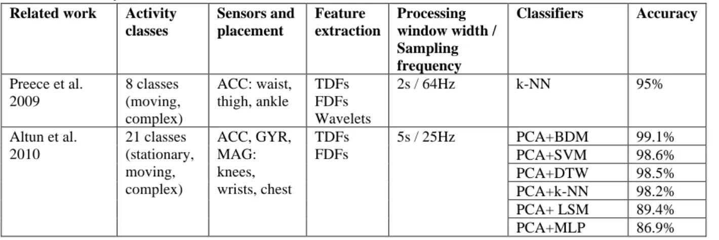
Table 1 summarizes the applied activity classes, sensor types and their placements, feature extraction modes, processing window widths, sampling frequencies, classification methods, and achieved accuracies in relevant works. The used abbreviations are described in the following subsections.
Table 1 Summary of relevant works Related work Activity
classes
Sensors and placement
Feature extraction
Processing window width / Sampling frequency
Classifiers Accuracy
Preece et al.
2009
8 classes (moving, complex)
ACC: waist, thigh, ankle
TDFs FDFs Wavelets
2s / 64Hz k-NN 95%
Altun et al.
2010
21 classes (stationary, moving, complex)
ACC, GYR, MAG:
knees, wrists, chest
TDFs FDFs
5s / 25Hz PCA+BDM 99.1%
PCA+SVM 98.6%
PCA+DTW 98.5%
PCA+k-NN 98.2%
PCA+ LSM 89.4%
PCA+MLP 86.9%
4
PCA+CT 81.0%
Lee et al. 2011 6 classes (stationary, moving, complex)
ACC: chest TDFs FDFs
10s / 20Hz LDA+MLP 94.43%
Zhu and Sheng 2011
8 classes (stationary, transitional, moving)
ACC: right thigh
TDFs 1s / 20Hz MLP+HMM 80.88%
Fuentes et al.
2012
4 classes (stationary, transitional)
ACC: chest TDFs 1s / 100Hz SVM 94.73%
Varkey et al.
2012
6 classes (stationary, moving, complex)
ACC, GYR:
right wrist, right foot
TDFs 1.6s / 20Hz SVM 97.2%
Martin et al.
2013
6 classes (stationary, moving, complex)
ACC, GYR, MAG:
multiple places
TDFs FDFs
3s / 6.25Hz (ACC), 100Hz (GYR), 7.69Hz (MAG)
CT 97%
Decision table 88%
NBC 78%
Chernbumroong et al. 2014
13 classes (moving, complex)
ACC, GYR:
dominant wrist
TDFs FDFs
3.88s / 33Hz SVM 97.2%
MLP 96.73%
RBF 95.67%
Li et al. 2014 6 classes (stationary, moving, complex)
ACC: waist TDFs 1s / 10Hz MLP 98.3%
k-NN 94.1%
Attal et al. 2015 12 classes (stationary, transitional, moving)
ACC: chest, right thigh, left ankle
TDFs FDFs Wavelets
1s / 25Hz k-NN 99.25%
Random forest 98.95%
SVM 95.55%
SLGMM 85.05%
HMM 83.89%
GMM 75.60%
k-means method 72.95%
Suarez et al.
2015
6 classes (stationary, moving)
ACC, GYR:
waist
TDFs 0.64s, 1.28s, 2.56s / 50Hz
Lazy learner 99%
CT 97%
Rule-based classifier
97%
NBC 84%
Korpela et al.
2016
5 classes (moving, complex)
ACC: right wrist
TDFs FDFs
1s / 100Hz CT 97.8%
2.1 Activity classes
In the related work, many activity classification approaches were used. The most widely used activities were standing and walking, which can be found in almost all works. Besides standing, other stationary activities can also be found in the literature, such as lying (Lee et al. 2011), sitting (Yang et al. 2009; Martin et al. 2013;
Ugolotti et al. 2013), or both (Altun et al. 2010; Zhu and Sheng 2011; Attal et al. 2015; Suarez et al. 2015).
Different transitional movements were also parts of the activity classes in some works, e.g. sit-to-stand and stand-to-sit (Zhu and Sheng 2011; Ugolotti et al. 2013; Attal et al. 2015), lie-to-sit and sit-to-lie (Zhu and Sheng 2011), lie-to-stand and stand-to-lie (Ugolotti et al. 2013), or stopping after walking (Fuentes et al. 2012).
Regarding the classification of longer motional activities, various speeds and types of forward movements were also tested, such as slow, normal and rush walking (Martin et al. 2013), jogging (Preece et al. 2009; Yang et al.
2009; Varkey et al. 2012; Field et al. 2015), and running (Preece et al. 2009; Altun et al. 2010; Martin et al.
2013; Li et al. 2014; Korpela et al. 2016). Some works tried to differentiate different directions of an activity type, like level walking, walking downstairs and upstairs (Preece et al. 2009; Yang et al. 2009; Altun et al. 2010;
Lee et al. 2011; Attal et al. 2015; Suarez et al. 2015) or walking backwards (Field et al. 2015). Yang et al. 2009
5
recorded even continuous rotational movements, such as walking left-circle or right-circle, and turning left or right. Special complex activities were also parts of the constructed databases, e.g. falling (Ugolotti et al. 2013; Li et al. 2014), jumping (Preece et al. 2009; Yang et al. 2009; Altun et al. 2010), writing (Varkey et al. 2012), brushing teeth (Bao and Intille 2004; Korpela et al. 2016), eating and drinking (Bao and Intille 2004), sweeping the floor, lifting a box onto a table, bouncing a ball (Field et al. 2015), driving (Lee et al. 2011), cycling (Bao and Intille 2004; Altun et al. 2010), etc.
2.2 Sensors and placement
The accelerometer (ACC) is the most popular sensor for monitoring the motion of the human body. This sensor measures acceleration in one or more axes. As seen in Table 1, many researchers used only a single unit to achieve activity recognition, but they differed in the placement of the sensor. Others applied multiple sensors fixed to different parts of the body. Beside the works listed in Table 1, Ugolotti et al. 2013 applied a single accelerometer fixed to the chest, Gonzalez et al. 2015 applied two accelerometer-based data loggers, which were mounted on each wrist, while Bao and Intille 2004 applied five biaxial sensors placed on each subject’s right hip, dominant wrist, non-dominant upper arm, dominant ankle, and non-dominant thigh.
Gyroscopes (GYR), which measure angular velocity around one or more axes, are less popular in movement recognition applications, and are mostly used together with accelerometers. None of the related researches used only gyroscopes. Tri-axial accelerometers and gyroscopes used together provide six degrees of freedom (6DoF) sensor units. Yang et al. 2009 used measurement units containing a triaxial accelerometer and a biaxial gyroscope, and placed them to eight places on the body: the wrists, the ankles, the knees, the hip, and the left elbow.
The fusion of inertial sensors and magnetometers (MAG) is also reported in the literature. The magnetic sensors measure the Earth`s magnetic field, and thus, they are able to detect rotational movements compared to the magnetic north. Magnetic sensors are usually used together with the inertial sensors, which provides 9DoF measurement systems, but Maekawa et al. 2013 utilized only magnetometers for activity classification. The authors used sensor gloves with 9 magnetic sensors on both hands, and tried to classify simple (walking, running) and complex (shave, brush teeth, use electric toothbrush, etc.) activities. Lee and Cho 2016 applied the sensors of mobile phones for activity recognition, while Field et al. 2015 utilized an inertial motion caption system, comprised of 17 inertial sensors attached to different parts of the body. The 9DoF sensors were combined to get a global orientation through a Kalman Filter.
2.3 Feature extraction
As activity and movement recognition is a typical pattern recognition problem, feature extraction plays a crucial role during the recognition process. Sensor-based features can be classified into three categories: TDFs, frequency-domain features (FDFs), and features computed using time-frequency analysis.
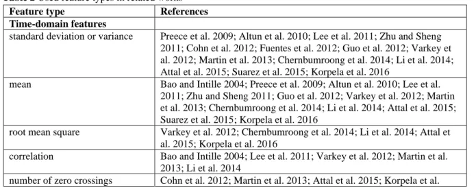
Most of the related researches used TDFs and/or FDFs. The type of features and their frequency of usage in references are shown in Table 2. It can be concluded that the most used TDFs are the mean and the standard deviation, and the most frequent FDFs are the spectral energy and the frequency-domain entropy.
Table 2 Used feature types in related works
Feature type References
Time-domain features
standard deviation or variance Preece et al. 2009; Altun et al. 2010; Lee et al. 2011; Zhu and Sheng 2011; Cohn et al. 2012; Fuentes et al. 2012; Guo et al. 2012; Varkey et al. 2012; Martin et al. 2013; Chernbumroong et al. 2014; Li et al. 2014;
Attal et al. 2015; Suarez et al. 2015; Korpela et al. 2016
mean Bao and Intille 2004; Preece et al. 2009; Altun et al. 2010; Lee et al.
2011; Zhu and Sheng 2011; Guo et al. 2012; Varkey et al. 2012; Martin et al. 2013; Chernbumroong et al. 2014; Li et al. 2014; Attal et al. 2015;
Suarez et al. 2015; Korpela et al. 2016
root mean square Varkey et al. 2012; Chernbumroong et al. 2014; Li et al. 2014; Attal et al. 2015; Korpela et al. 2016
correlation Bao and Intille 2004; Lee et al. 2011; Varkey et al. 2012; Martin et al.
2013; Li et al. 2014
number of zero crossings Cohn et al. 2012; Martin et al. 2013; Attal et al. 2015; Korpela et al.
6 2016
kurtosis Altun et al. 2010; Guo et al. 2012; Chernbumroong et al. 2014; Attal et al. 2015
range Fuentes et al. 2012; Varkey et al. 2012; Li et al. 2014; Attal et al. 2015 skewness Altun et al. 2010; Guo et al. 2012; Chernbumroong et al. 2014; Attal et
al. 2015
maximum Varkey et al. 2012;Chernbumroong et al. 2014; Suarez et al. 2015 minimum Chernbumroong et al. 2014; Suarez et al. 2015
number of rapid changes Cohn et al. 2012 magnitude of the first peak of the
autocorrelation
Cohn et al. 2012 Frequency-domain features
frequency-domain entropy Bao and Intille 2004; Preece et al. 2009; Lee et al. 2011; Martin et al.
2013; Chernbumroong et al. 2014; Attal et al. 2015
spectral energy Preece et al. 2009; Maekawa et al. 2013; Martin et al. 2013; Li et al.
2014; Attal et al. 2015; Korpela et al. 2016 magnitude of the defined first few
highest peaks
Preece et al. 2009; Guo et al. 2012; Maekawa et al. 2013;
Chernbumroong et al. 2014 frequency of the defined first few
peaks with highest amplitude
Altun et al. 2010; Guo et al. 2012; Maekawa et al. 2013 correlation between axes Preece et al. 2009; Chernbumroong et al. 2014
median frequency Cohn et al. 2012; Martin et al. 2013
DC component Attal et al. 2015
median power Cohn et al. 2012
principal frequency Preece et al. 2009
Using wavelet analysis, the signal is decomposed into a series of coefficients, which carry both spectral and temporal information about the original signal. Two works (Preece et al. 2009; Attal et al. 2015) tested this feature extraction method for the classification of activities. Preece et al. 2009 utilized the next features: the sum of the squared detail coefficients at different levels, the sum of the squares of the detail and wavelet packet approximation coefficients across different levels, the standard deviations and root mean square (RMS) values of detail and wavelet packet approximation coefficients at a few different levels, and the sum of the absolute values of coefficients at different levels. Attal et al. 2015 applied the following features: the sum of detail coefficients of wavelets, the sum of squared detail coefficients of wavelets, the energy of detail wavelets coefficients, and the energy of approximation wavelets coefficients.
2.4 Processing window width and sampling frequency
Windowing plays also a very important role during the extraction of features. Usually features are computed in fixed-size windows, which are shifted also with a fixed time. In the related work, the width of the applied processing windows is between 1s and 10s, and the smallest size, 0.64s, was tested by Suarez et al. 2015. The sampling frequency is also a very important factor in the processing phase. In relevant works, the applied frequencies were between 10Hz and 100Hz.
2.5 Classifiers
The classification of the defined activities using the computed feature vectors can be done using different classification methods. As shown in Table 1, the most popular classifiers in relevant works are: support vector machines (SVM), the k-nearest neighbor (k-NN) method, decision trees or classification trees (CT), the naïve Bayes classifier (NBC), and multi-layer perceptron (MLP) neural networks. Some other methods were also tested, as radial basis function (RBF) neural networks, the least-squares method (LSM), Bayesian decision making (BDM), dynamic time warping (DTW), decision table, rule-based classifier, Gaussian mixture modeling (GMM), supervised learning GMMs (SLGMM), the k-means method, random forest, lazy learner, and hidden Markov models (HMMs). In some researches, the classifiers were used together with some dimension reduction methods. The most common methods are the principal component analysis (PCA) and the LDA. Guo et al. 2012 applied the generalized discriminant analysis (GDA) method with the multiclass relevance vector machine classifier. Some researchers even tested two different classification methods together: neural networks and
7
HMMs (Zhu and Sheng 2011), hierarchical temporal memories and SVMs (Ugolotti et al. 2013), CTs and HMMs (Maekawa et al. 2013), k-means clustering and HMMs (Lee and Cho 2016).
3 Experimental setup
The sensor devices used in body sensor networks must be designed with the aim of providing the highest degree of mobility for the patients. They must be small, lightweight, and wireless wearable units.
The used prototype system, which can be seen in Fig. 1 consists of an IRIS WSN mote, and a 9DoF digital sensor board connected to it. The IRIS mote is equipped with an Atmel ATmega 1281L 8-bit microcontroller, and an RF231 IEEE 802.15.4 compatible radio transceiver. The current draw of the microcontroller is 8mA in active mode, and 8µA in sleep mode, while the radio transceiver consumes 17mA during transmission, and 16mA during reception. The maximal data throughput of the radio transceiver is 250kbps, and its outdoor range is over 300m. The connected 9DoF sensor board is made up of an ADXL345 tri-axial MicroElectroMechanical System (MEMS) accelerometer, an ITG3200 tri-axial MEMS gyroscope, and an HMC5883L tri-axial magnetoresistive technology-based magnetometer. The ADXL345 is a low power accelerometer (the current draw is 40µA in measurement mode, and 0.1µA in sleep mode), which can measure up to ±16g in 13-bit resolution with the highest sampling rate of 3.2kHz. The gyroscope features a 16-bit analog-to-digital converter, and it can measure angular rate in a range of ±2000deg/s with 8kHz frequency. The normal operating current of the gyroscope is 6.5mA, while the sleep mode current is 5µA. The measurement range of the magnetic sensor is
±8.1Ga in 12-bit resolution with 160Hz maximal sampling rate, and it consumes 2µA current draw in idle mode, while 100µA in measurement mode.
A TinyOS-based driver was developed and implemented to configure the sensors and cyclically read the measurement data. The data are read from the sensors via the I2C interface, and sent via wireless communication to a BaseStation mote, which uses serial communication to forward the data to a PC.
3.1 Data acquisition
Eleven activities were defined in order to recognize specific arm movements in stationary positions and also during the movement of the body. The used activities are the following:
1. “standing without movement of the arms”, 2. “sitting with the arms resting on a table”, 3. “walking”,
4. “turning around in one place”, 5. “jogging”,
6. “raising and lowering the left arm during standing”, 7. “raising and lowering the right arm during standing”, 8. “raising and lowering both arms during standing”, 9. “raising and lowering the left arm during walking”, 10. “raising and lowering the right arm during walking”, 11. “raising and lowering both arms during walking”.
Data were collected with the help of nine male subjects (ages between 20 and 50, and height between 165cm and 190cm) for all activities. The IRIS motes with the attached 9DoF sensor motes were mounted on each wrist of the subjects. The data were recorded in fixed-length sessions of 20s for all activities using 125Hz sampling frequency, which means 2500 measurements per sensor. The measurements were performed in a laboratory environment.
4 Classification algorithm
The classification is performed in four main stages. The software architecture with the four stages can be seen in Fig. 2. In the first step, the measurement data are preprocessed (Stage I.). In the second stage (Stage II.) features are extracted from the signals on each unit. Possible aggregation of the extracted features is also done in this stage. The proposed algorithm assumes the transmission of the vector of the extracted features from one mote to the other, and the rest of the algorithm should be implemented in the microcontroller of the receiving device.
Dimension reduction is done in the third stage (Stage III.), while classification is performed in the fourth stage (Stage IV.). Two different algorithms were applied and tested. In the first type, the third stage is not performed, and the classifiers receive the feature vectors directly, while in the second case the data sets are dimensionally
8
reduced, so the classifiers have less input parameters. The advantage of the dimension reduction method is that it removes the redundant information.
4.1 Preprocessing 4.1.1 Error compensation
Due to high error rates caused by structural errors of the sensors, the raw measurements were compensated in the preprocessing phase. The calibration parameters (scale factors, offsets, and non-orthogonality errors) were obtained using an offline evolutionary algorithm-based method (Sarcevic et al. 2014). For the computation of the parameters, the algorithm uses measurements recorded in multiple stationary orientations.
4.1.2 Windowing
The extraction of feature values is performed in fixed-size segments, which are shifted with constant sizes. To generate a high number of input vectors, small window shifts were used. For hardware implementation, the size of the shifts depends on the available resources and the required response time, since the algorithm updates the movement classes after each window shift, and the reduction of the size of the shifts increases the necessary computation performance.
Both the CPU computation performance and the power resources are limited in IRIS WSN motes, so it is important to minimize the usage of these resources while maximizing the recognition efficiency. The required computation performance and the current draw of the sensors can be reduced if the sampling frequency is decreased.
4.2 Feature extraction 4.2.1 Feature types
The used features were chosen by their memory usage, required computation, and possible quantity of information. Due to easy implementation and low memory usage, only time-domain analysis was performed on the signals. Many of the chosen features were previously used for EMG pattern recognition (Phinyomark et al.
2012), and to the best knowledge of the authors, most of them were not applied previously for movement classification. The used TDFs require only one or two previous measurements, so there is no need to store all the measurement data in the window as it is required for frequency domain analysis. But even standard deviation, which is the most frequently used features, requires the storage of the measurement vector in the window, since first the average needs to be calculated. The following TDFs were chosen for this research:
• Mean Absolute Value (MAV): The calculation of the MAV feature can be expressed as follows, MAV =1
𝑁∑𝑁𝑖=1|𝑥𝑖|, (1)
where N is the number samples in the window, and xi are the signal amplitudes at the given index.
• Willison Amplitude (WAMP): The number of amplitude changes of incoming signals within a window, which are higher than a given threshold level. The computation of the WAMP can be expressed as WAMP = ∑𝑁−1𝑖=1[𝑓(𝑥𝑖− 𝑥𝑖+1)], 𝑓(𝑥) {1, if(𝑥 ≥ 𝑡ℎ)
0, otherwise, (2)
where th is the threshold, which is the peak-to-peak noise level.
• Number of Zero Crossings (NZC): The number of times when the amplitude values cross the zero- amplitude level, and the difference between the values with opposite signs is larger than a defined threshold. The computation of the NZC feature can be represented as
NZC = ∑𝑁−1𝑖=1[𝑠𝑔𝑛(𝑥𝑖∙ 𝑥𝑖+1) ∩ |𝑥𝑖− 𝑥𝑖+1| ≥ 𝑡ℎ], 𝑠𝑔𝑛(𝑥) = {1, if(𝑥 ≥ 0)
0, otherwise (3)
• Number of Slope Sign Changes (NSSC): The number of direction changes, where among the three consecutive values the first or the last changes are larger than the predefined limit. The computation of this feature can be represented as follows,
NSSC = ∑𝑁−1𝑖=2[𝑓[(𝑥𝑖− 𝑥𝑖−1) ∙ (𝑥𝑖− 𝑥𝑖+1)]], 𝑓(𝑥) = {1, if(𝑥 ≥ 𝑡ℎ)
0, otherwise (4)
• Maximal (MAX) and Minimal (MIN) value: The highest and lowest measured value in the processing window.
9
• RMS: The calculation of the RMS in a processing segment can be done as RMS = √1
𝑁∑𝑁𝑖=1𝑥𝑖2 (5)
• Waveform Length (WL): The cumulative length of the waveform over the time segment, which is calculated by the sum of absolute changes between two measurements:
WL = ∑𝑁−1𝑖=1|𝑥𝑖+1− 𝑥𝑖| (6)
4.2.2 Extraction modes
The used input vectors were generated and tested with the use of two TDF calculation modes:
• Separately used axes (SEP): The features are extracted separately for the X, Y, and Z axes of the sensors.
• Vector magnitude-based (VL): The changes in the vector length are used for the computation of the TDFs.
The advantages of this feature extraction mode are that three times less features are generated than with the SEP mode, and that it should be less sensitive to slight differences between movements of different subjects, or small displacements of the sensor motes on the wrists. However, it should not be able to recognize different poses in stationary positions. The magnitude-based feature extraction cannot provide valuable information in case of the magnetometer measurements, because the magnitude of the magnetic field is constant in ideal situations, thus, any measured distortions are caused by the changes in the indoor environment. Using the other two sensor types, the accelerometer and the gyroscope, this feature extraction mode can provide important information for the classification process. Except the NZC feature, which cannot give helpful information, since the magnitude cannot be negative, all other of the previously described TDF types can be effective.
4.2.3 Feature aggregation
The usage of the separately extracted features for the three sensor axes can result in a very high number of features, which can increase the complexity of the classification algorithm. Also, it can have a negative effect on the recognition efficiency if the subjects do not fix the units correctly to their wrists. A possible solution to both previous problems can be the aggregation (AGG) of the separately computed features. As expressed in Eq. 7, this can be done by calculating a linear combination of the feature values computed for each axis for a specific feature type.
𝑓𝑒𝑎𝑡𝐴𝐺𝐺 = 𝑤𝑋∙ 𝑓𝑒𝑎𝑡𝑋+ 𝑤𝑌∙ 𝑓𝑒𝑎𝑡𝑌+ 𝑤𝑍∙ 𝑓𝑒𝑎𝑡𝑍, (7)
where featAGG is the aggregated feature value, featX, featY, and featZ are the extracted features for each axis, and wX, wY, and wZ are the corresponding weights.
4.3 Dimension reduction
The LDA method was used to perform dimensionality reduction on the datasets, which is a widely-used subspace learning method in statistics, pattern recognition and machine learning. This method aims to seek a set of optimal vectors, denoted by 𝑾 = [𝒘1, 𝒘2, … , 𝒘𝑚] ∈ ℜ𝑑x𝑚, projecting the d-dimensional input data into an m-dimensional subspace, such that the Fisher criterion is maximized (Martinez and Kak 2001; Gu et al. 2011).
The Fisher criterion, given in Eq. 8, aims at finding a feature representation, by which the within-class distance is minimized and the between-class distance is maximized.
arg max𝑾tr((𝑾𝑇𝑺𝑤𝑾)−1(𝑾𝑇𝑺𝑏𝑾)) ()
where Sb and Sw are the between-class scatter matrix and the within-class scatter matrix respectively, and are defined as
𝑺𝑤= ∑𝑐𝑗=1∑𝑁𝑖=1𝑗 (𝒙𝑖𝑗− 𝝁𝑗)(𝒙𝑖𝑗− 𝝁𝑗)𝑇 ()
𝑺𝑏= ∑𝑐𝑗=1(𝝁𝑗− 𝝁)(𝝁𝑗− 𝝁)𝑇 ()
where 𝑥𝑖𝑗 represents the i-th sample of class j, µj is the mean vector of class j, c is the number of classes, Nj is the number of samples in class j, and µ is the overall mean vector of all classes. The mean vector of a class and the overall mean vector can be calculated as follows,
10 𝝁𝑗= 1
𝑁𝑗∑𝑁𝑖=1𝑗 𝒙𝑖𝑗 ()
𝝁 =1
𝑐∑𝑐𝑗=1∑𝑁𝑖=1𝑗 𝒙𝑖𝑗 ()
The solution to the problem of maximizing the Fisher criterion is obtained by an eigenvalue decomposition of 𝑺𝑤−1𝑺𝑏, and taking the eigenvectors corresponding to the highest eigenvalues. There are c-1 generalized eigenvectors. If the number of features is less than c-1, then the number of eigenvectors will be equal to the number of features.
4.4 Classification methods
In this research seven possibly applicable classification methods were chosen and tested:
• Nearest Centroid Classifier (NCC): The NCC is used in various areas of pattern recognition because it is simple and fast. The method determines the Euclidean distance from an unknown object to the centroid of each class, and assigns the object to the class with the shortest distance. The Euclidean distance between the 𝑥𝑖∈ ℜ𝑛 feature vector and the n-dimensional mj vector of mean values for class j can be calculated as
𝑑𝑖𝑠𝑡(𝒙, 𝒎𝑗) = √∑𝑛𝑖=1(𝑥𝑖− 𝑚𝑗𝑖)2 ()
• MLP: Artificial Neural Networks (ANNs) are inspired by the animal`s brain, and are used to approximate target functions (Mitchell 1997). The MLP is a feedforward ANN, where neurons are organized into three or more layers (an input and an output layer with one or more hidden layers), with each layer fully connected to the next one using weighted connections. A neuron has an activation function that maps the sum of its weighted inputs to the output. The oj output of one node can be defined as
𝑜𝑗 = 𝑓(𝒗𝑗∙ 𝒙 + 𝑏) ()
where x is the input vector, vj is the vector containing the weights, b is the bias value, and f is the applied activation function.
Most commonly MLP networks are trained using the backpropagation algorithm, which employs gradient descent to attempt to minimize the squared error between target values and the network output values.
• NBC: The NBC is a highly practical Bayesian learning method. It is based on the simplifying assumption that, given the target value of the instance, the attribute values are conditionally independent, and the probability of observing the conjunction for attributes is just the product of the probabilities for the individual attributes (Mitchell 1997). Eq. 15 presents the approach used by the NBC.
𝜐𝑁𝐵 = arg max𝜐𝑗∈𝑉𝑃(𝜐𝑗) ∏ 𝑃(𝑎𝑖 𝑖|𝜐𝑗) ()
where υj denotes the target value output of the classifier, V is the finite set of target values, ai are the attribute values, and P(υj) are the probabilities of υj target values.
• SVM: In SVMs, a data point is viewed as a p-dimensional vector, and the goal is to separate such points with (p-1)-dimensional hyperplanes (Varkey et al. 2012). The hyperplane can be defined as
𝐹(𝒙) = 𝒘 ∙ 𝒙 + 𝑏, (16)
where x is the vector to be recognized, w is the normal vector to the hyperplane, and b determines the offset from the origin along the normal vector. Eq. 17 defines the normal vector, and is subject to the condition expressed in Eq. 18.
𝒘∗= ∑𝑙𝑖=1𝛼𝑖∗∙ 𝑦𝑖𝒙𝑖, (17)
where αi is the i-th Lagrange multiplier, 𝑦𝑖∈ {−1,1}, and l is the number of support vectors.
𝛼𝑖∗[𝑦𝑖(𝒘∗𝑇𝒙𝑖+ 𝑏∗) − 1] = 0, ∀𝛼𝑖≠ 0 (18)
The function of the hyperplane is not suitable for solving linearly non-separable problems, or dealing with more than two classes. To classify data into multiple classes, two common methods can be used: “one-
11 versus-one” (OvO) and “one-versus-all” (OvA).
• k-NN: The k-NN algorithm classifies the objects based on the closest training examples in the feature space (Altun et al. 2010; Li et al. 2014). To classify a new observation, the method finds the k nearest samples in the training data, and assigns the new sample to the class which provides the most neighbors.
The Euclidean distance measure is used.
• CT: The CT is a rule-based algorithm, which uses a tree-like set of nodes for classifying inputs (Altun et al. 2010; Martin et al. 2013). The tree has predefined conditions at each node of the tree, and makes binary decisions based on these rules. The condition of the following node is checked until a leaf is found that contains the classification result.
5 Performance evaluation
Altogether 340 datasets were constructed using different combinations of used sensor types, TDF calculation modes, processing window sizes, and sampling frequencies.
The cost of the system can be decreased by decreasing the number of used sensor types, but in recognition efficiency their fusion can result in a drastic improvement. In order to explore the effect of the used sensor types in the application, seven sensor combinations were defined, since the three sensor types can be used alone, in pairs, and together. The SEP and AGG feature extraction modes were tested for all seven sensor combinations, while the VL mode was used only for the accelerometer and the gyroscope alone, and their data used together, since, as described in Sect. 4.2, the magnetometer data cannot provide valuable information using this feature extraction mode. Thus, 17 combinations were constructed using the applied sensor types and feature extraction modes.
The use of large processing windows can increase the required computation, and it can make harder the detection of transitions between activities. Since one of the goals of this research is to explore the recognition efficiency using processing windows in millisecond range, the following window width and shift pairs were tested: 80ms width and 40ms shift; 200ms width and 40ms shift; 400ms width and 80ms shift; 800ms width and 80ms shift.
The necessary computation can be lowered by decreasing the sampling frequency, but it can have a negative effect if any important spectral components disappear. The spectral analysis of the obtained measurements shows, that in case of the accelerometer and the gyroscope, the highest frequencies of the dominant spectral components are below 15Hz, while in the case of the magnetometer data, no higher components can be noticed above 5Hz. To find the optimal setup, where the chosen TDFs can be still effective, datasets were generated using five sampling frequencies: 25Hz, 50Hz, 75Hz, 100Hz, and 125Hz. The data for the four lower frequencies were obtained by downsampling the measurement data collected with 125Hz sampling frequency.
Data from five of the nine subjects were used for the training of the classifiers, while the data from the remaining four subjects were tested as unknown inputs for the validation of the trained classifiers. All six classification techniques were tested for all datasets with and without dimension reduction. No results could be achieved using the NBC without LDA, since some classes have features with zero variance.
In this study both the OvA and the OvO methods were tested and used for comparison in case of the SVM classifier.
The k-NN classification algorithm was tested with 1 to 10 neighbors. Analyzing the efficiencies on validation data, without dimension reduction a convergence (97%) can be noticed at 1-2 neighbors in almost 55% of the setups, while other setups mostly converge at 3-4 neighbors. With LDA 1-4 neighbors are needed to achieve convergence as well, but in most cases 4 neighbors are necessary.
The training of the MLP was tested using 1 to 15 neurons in the hidden layer. The 70% of the training data were used as training inputs, and 30% as validation inputs for the training method. The validation datasets were used as unknown inputs for testing the efficiency of the classifier. Hyperbolic tangent sigmoid transfer function was used in the hidden layer, while the neurons in the output layer were created using the linear transfer function. The scaled conjugate gradient method was used for training. The results show that in both cases (with and without using LDA), at least 9 hidden layer neurons are needed to achieve convergence (97%), and in more than 70% of the setups 9-12 neurons were required. It can be also noticed, that without dimension reduction the distribution of the converge points is equal, while with LDA more setups converge at 9-10 neurons.
In the further comparison, the authors used the setup with the highest recognition rate on unknown samples
12 for both the k-NN and the MLP algorithms.
5.1 Efficiency comparison of the classification methods
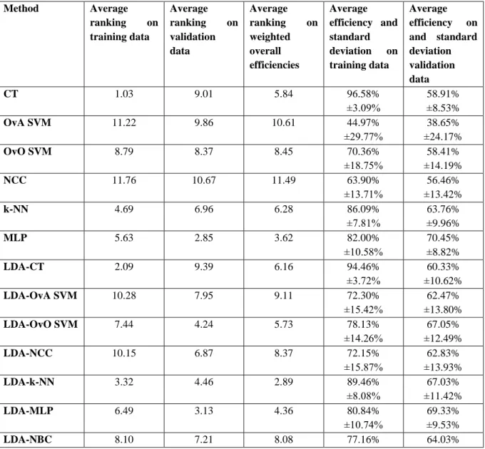
Table 3 summarizes the average rankings of the thirteen classification methods on training and validation data, and on weighted overall efficiencies. Since it is important to classify both the known and the unknown data correctly, the weighted efficiency was calculated using the sum of the achieved recognition rates on known and unknown data, but the efficiency on validation data was used with a double weight. The average ranking was computed using the ranking order of the methods for each of the 340 setups. The average efficiencies are also presented in Table 3. Comparing the rankings on validation data, it can be stated, that the MLP and the LDA- MLP methods are the most powerful classifiers. The MLP was the best in almost 48% of the datasets, and its average ranking is 2.85, while the average ranking of the LDA-MLP is 3.13. The NCC method achieved the worst results with an average of 10.67, but the LDA-CT, CT and OvO SVM methods had also poor results with a ranking above 9. The results obtained only on training data show, that the CT and the LDA-CT provide the highest results, with an average recognition rate of 96.58% and 94.46% respectively. They are followed by the LDA-k-NN (89.46%) and the k-NN (86.09%) algorithms. These classification techniques are designed to best fit on training data, but are not too efficient on unknown data. The MLP, which proved to be the best method in case of validation data, provided 82.00% efficiency on known datasets, and was fifth in the rankings. Analyzing the overall recognition, it can be seen, that the LDA-k-NN is the best classifier with an average ranking of 2.89.
This method is followed by the MLP (3.62) and the LDA-MLP (4.36).
Table 3 Average ranking and efficiency of different classification methods on different data types
Method Average
ranking on training data
Average ranking on validation data
Average ranking on weighted overall efficiencies
Average efficiency and standard deviation on training data
Average efficiency on and standard deviation validation data
CT 1.03 9.01 5.84 96.58%
±3.09%
58.91%
±8.53%
OvA SVM 11.22 9.86 10.61 44.97%
±29.77%
38.65%
±24.17%
OvO SVM 8.79 8.37 8.45 70.36%
±18.75%
58.41%
±14.19%
NCC 11.76 10.67 11.49 63.90%
±13.71%
56.46%
±13.42%
k-NN 4.69 6.96 6.28 86.09%
±7.81%
63.76%
±9.96%
MLP 5.63 2.85 3.62 82.00%
±10.58%
70.45%
±8.82%
LDA-CT 2.09 9.39 6.16 94.46%
±3.72%
60.33%
±10.62%
LDA-OvA SVM 10.28 7.95 9.11 72.30%
±15.42%
62.47%
±13.80%
LDA-OvO SVM 7.44 4.24 5.73 78.13%
±14.26%
67.05%
±12.49%
LDA-NCC 10.15 6.87 8.37 72.15%
±15.87%
62.83%
±13.93%
LDA-k-NN 3.32 4.46 2.89 89.46%
±8.08%
67.03%
±11.42%
LDA-MLP 6.49 3.13 4.36 80.84%
±10.74%
69.33%
±9.53%
LDA-NBC 8.10 7.21 8.08 77.16% 64.03%
13
±13.66% ±11.64%
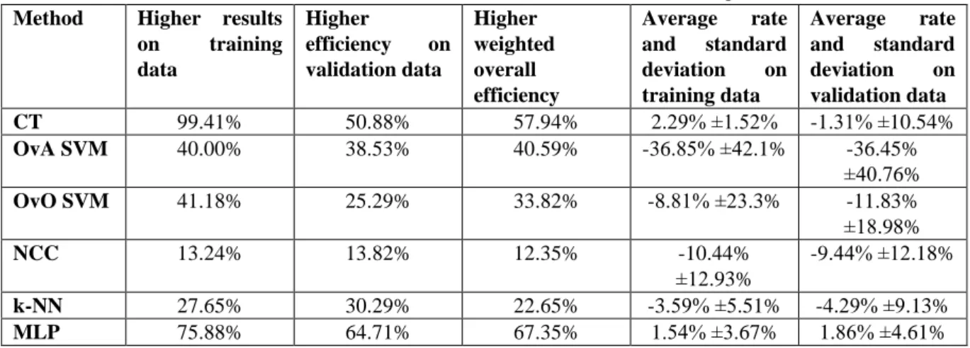
Rates for the 340 datasets when the tested classification techniques performed better without LDA, and the average rate of differences are tabulated in Table 4. It can be observed, that the LDA-based dimension reduction has in overall a slight negative effect on the efficiency of the MLP. It decreases the efficiency in around 70% of the datasets, but the differences are not significant. Also, very small differences can be noticed for the CT, but the dimension reduction decreases the ability to recognize known data for almost all setups, while in around half of the datasets it increases the overall efficiency and the recognition rate on validation data. The LDA method has a very positive effect on the other classification techniques. The most significant improvement was achieved with the NCC method, for which the application of dimension reduction increased the recognition rates in average by 10%. The obtained efficiencies were also higher in around 87% of the setups for all three compared result types. For the other three algorithms, higher classification rates were achieved in around 60-70% of the datasets both on training and validation data. The highest effect can be noticed on the OvA SVM, since without dimension reduction almost 37% lower efficiencies were obtained for both known and unknown data.
Table 4 Effect of LDA-based dimension reduction on the tested classification techniques Method Higher results
on training data
Higher
efficiency on validation data
Higher weighted overall efficiency
Average rate and standard deviation on training data
Average rate and standard deviation on validation data
CT 99.41% 50.88% 57.94% 2.29% ±1.52% -1.31% ±10.54%
OvA SVM 40.00% 38.53% 40.59% -36.85% ±42.1% -36.45%
±40.76%
OvO SVM 41.18% 25.29% 33.82% -8.81% ±23.3% -11.83%
±18.98%
NCC 13.24% 13.82% 12.35% -10.44%
±12.93%
-9.44% ±12.18%
k-NN 27.65% 30.29% 22.65% -3.59% ±5.51% -4.29% ±9.13%
MLP 75.88% 64.71% 67.35% 1.54% ±3.67% 1.86% ±4.61%
5.2 Efficiency comparison of the tested sampling frequencies and processing window sizes
The further comparison of the results, achieved with different sampling frequencies and window sizes, was done using the best achieved overall weighted efficiencies.
The results show, that using the five tested sampling frequencies, the average difference between the highest and lowest efficiencies is 6.74% ±8.47% for training data, and 6.83% ±6.45% for validation data. The impact of increasing the sampling frequency is almost the same for the four different processing window sizes, but it has different effect on the 17 combinations of extraction modes and used sensors. Analyzing results on validation data, larger differences can be noticed when the magnetometer is used alone. In case of the SEP mode, the difference between the largest and smallest efficiency is 3-7%, and the recognition rate is decreasing with the increasing of the sampling frequency. The other setups provide almost constant efficiency or a rising tendency by increasing the sampling frequency. The AGG setup provides differences between 2.5% and 4.5% using only the magnetometer data, and around 3% for the data of the angular velocity sensor. Higher differences, can be also observed when the SEP feature extraction is performed on the fused data of the magnetic sensor and the gyroscope (3-5.7%), when the AGG features are applied on the data of the magnetometer and the accelerometer together (2.5-8%), and when the data of the accelerometer and gyroscope are used together and VL-based feature extraction is done (3.2-6%). The other setups provided below 2% differences.
The size of the processing window width has a more significant effect on recognition rates, since the larger windows always result in higher efficiency. In overall, the highest classification efficiencies are higher than the lowest rates for 13.24% ±6.34% on training data, and 28.1% ±14.48% on validation data. The improvements do not differ greatly for different sampling frequencies, but they are more significant in case of the 17 different combinations of sensors and feature extraction modes. Especially high differences on validation data can be noticed for the three setups when the VL-based feature computation was used: gyroscope – 27.6-29.2%, accelerometer – 18.7-27%, and the gyroscope and the accelerometer together – 26-28.6%. The lowest
14
improvements can be observed in case of the two setups when the three sensors were used together: SEP – 9.7- 11.1%, AGG – 7.1-9.5%. The increasing of the window size also has lower effect in case of the gyroscope when the features are computed using the SEP and AGG methods, 11.5-12.5% and 6.4-12.5% respectively, and when the SEP technique is used on the fused data of the gyroscope and the accelerometer, where the differences are between 10.4% and 12.8%.
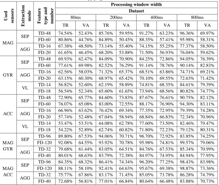
5.3 Efficiency comparison of the tested feature extraction modes and sensor combinations
The best results for the 17 different combinations in the four different processing window widths can be seen in Fig 3. It can be observed, that using only the magnetic sensor with the AGG feature extraction can provide the lowest recognition rates, since with the smallest window size only 39.95% can be achieved, while with even the largest processing window the efficiency increases only to 60.05%. Using the SEP mode, the recognition rates are much higher, 57.03% with the 80ms window and 67.18% with the 800ms window size.
Using only the angular rate sensor provides the highest results with the SEP method: 66.6-80.7%. The VL mode provides smaller classification rates, but the difference decreases by increasing the size of the processing window, since with the smallest window size the difference is 20%, while with the largest window a recognition rate of 78.33% can be achieved, which is only 2.37% lower than with the SEP mode. The number of features was 48 for the SEP mode and 14 for the VL mode, which is a significant difference. Using the AGG extraction mode, for which the size of the feature vector was 16, significant difference to the VL mode can be noticed for the smaller window sizes. The recognition efficiency was 8,5% higher for the 80ms window, and 10,18% for the 200ms window, but for the two larger sizes the VL achieved better results, 2.55% and 9.57% respectively.
Using only the accelerometer, similar results can be achieved as with the gyroscope. For the two smaller windows with the SEP and AGG modes the accelerometer performed lower results, while with increasing the window size, the accelerometer provides higher efficiencies than the gyroscope. For the SEP mode, the differences were 1-3%, but for the two smaller windows with the AGG mode the recognition rates are lower for 3-5%, and higher for the two larger windows for 7%. With the VL-based feature vectors the accelerometer provides better results. Using the 80ms processing window size the difference was around 10%, but the difference decreases, and was only 1% for the 800ms window.
The usage of the magnetometer itself cannot provide usable results, but it can improve the performance of the inertial sensors, since the largest classification rates are 85.03% and 87.2% respectively. In case of the gyroscope, in average, the results were improved for 3.26% ±3.59% for the SEP mode, while with the accelerometer it provides an improvement of 5.11% ±3.19% for the SEP, and 7.45% ±7.44% for the AGG mode.
For the setup where the data from the magnetometer and the gyroscope were fused, and the AGG feature extraction mode was performed, in average the results were even slightly lower than when the data from the gyroscope was used alone.
The highest recognition rate on validation data, 89.14% (99.48% on training data), was reached using all three sensor types with the SEP feature extraction in the largest processing window. This setup requires the usage of 144 features. With the same extraction mode, but without using the magnetic sensor, 87.96%
classification efficiency can be achieved on validation data, and 98.91% on training data, with a required feature number of 96. By decreasing the size of the processing window, the classification rate significantly decreases, but even with the smallest window, an efficiency of 77.32% can be achieved with, and 76.5% without the magnetometer. The difference between these two setups is a little above 1% in efficiency, but the number of features, the energy consumption, and the cost are all increased if the magnetic sensor is added to the system.
Similar differences can be noticed with the AGG extraction mode also.
The setup where the features were computed using the VL-based extraction, and the data from the angular velocity sensor and the accelerometer were used together, also proved to be very useful. The feature vectors consisted of 28 different features, and with the largest processing window the recognition rate was 86.17%. This extraction mode fails when the processing windows are small, since the efficiency with the 80ms size was only 55.8%, and the AGG-based features provide higher efficiencies in these cases.
5.4 Training time comparison of the classification methods
Training time is not a crucial factor for the implementation of a classifier, but it can prove to be very important, especially when different combinations of features should be tested. To generate comparable data, all trainings were done on the same PC with the next characteristics: Intel core i7 3.5GHz processor, 16GB RAM, GeForce
15 GTX 770 video card.
The computation of the LDA matrices proves to be very fast, and even for the largest setup, which contains 144 inputs, less than 1.8s is required.
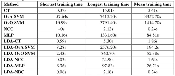
The k-NN method does not require any training, since it uses the entire dataset for the classification. The shortest, longest, and mean training times for the other classification methods are summarized in Table 5. It can be stated, that the most time consuming from the tested classification methods is the OvA SVM algorithm, since the training of the larger setups can last for more than 2 hours, but even the shortest time was almost 1 minute.
The OvO SVM method proves to be much faster, but the longest time is still above 1 hour, while the shortest is 17s. The dimension reduction has a significant impact on the SVM-based methods, since it decreases the training time by 93.51% ±11.4% for the OvA, and by 92.45% ±10.79% for the OvO method. Beside the high reduction in training time, caused by the LDA, the longest required intervals are still too high for both methods. The training of the CT method requires between 0.37-15s, and the LDA method does not reduce the training time for all setups, but the longest training was three times shorter than without the dimension reduction. The computation of the parameters for the NCC classifiers is very low for low dimension setups, but for the largest setups it can last for even 25s. The effect of the LDA can be noticed only at the larger setups, and it reduces the maximal time to 2s. The training of the LDA-NBC classification method, similarly to the LDA-NCC, lasts between a few hundredths and 2s. The training of the MLP classifiers is also very time-consuming. The longest interval using 10 hidden layer neurons was 1331.6s. Besides, that even the length of only one training is long, to find the optimal setup, multiple trainings are required with different neuron numbers in the hidden layer. This significantly increases the required training time. The LDA-based dimension reduction has a significant effect on this classification method, since it reduces the longest training time to 97.83s, and in average it reduces the training time by 48.43% ±34.92%.
Table 5 Smallest, highest, and mean required training times of the tested classification methods Method Shortest training time Longest training time Mean training time
CT 0.37s 15.01s 3.41s
OvA SVM 57.64s 7415.20s 3352.70s
OvO SVM 16.99s 3791.40s 1414.70s
NCC ~0s 2.12s 0.24s
MLP 10.16s 1331.60s 84.81s
LDA-CT 0.59s 5.30s 1.86s
LDA-OvA SVM 8.28s 2576.20s 194.2s
LDA-OvO SVM 2.43s 860.70s 52.38s
LDA-NCC 0.03s 24.90s 1.64s
LDA-MLP 6.36s 97.83s 26.71s
LDA-NBC 0.06s 2.18s 0.34s
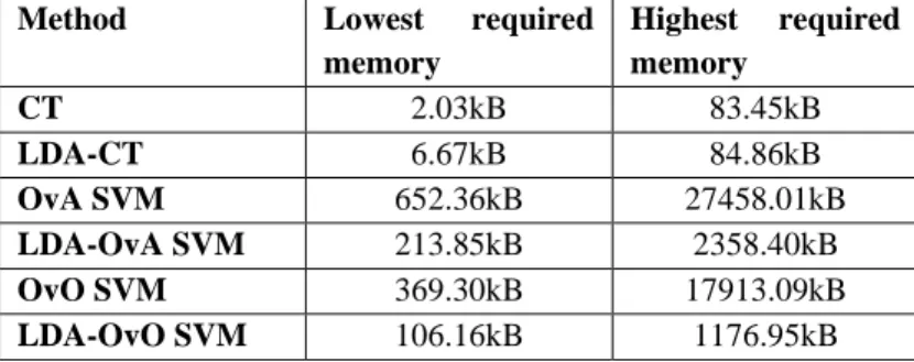
5.5 Memory requirement comparison of the classification methods
The required space for the implementation of a classifier is a very important factor, since microcontroller-based systems have limited amounts of memory.
The required number of parameters for the implementation of the NBC, the NCC, and the MLP classifiers can be calculated using the number of features and classes. The number of hidden layer neurons is also needed in case of the MLP-based methods. In case of the k-NN, the number of samples in the classes is required, since the algorithm uses the entire feature set to determine the class. The required memory for the SVMs and the CTs cannot be calculated as a function of the number of features and classes, because the number of necessary support vectors in case of SVMs and necessary nodes in case of CTs differs. For comparison, the required memory spaces were calculated in bytes (1 floating-point number is equal with 4 bytes).
The LDA projection matrices have 10 rows, because 11 classes are used, and the number of columns is equal to the number of features. If the number of features is less than 10, the number of rows will be equal to the number of features.
The training of the NCC was performed by calculating the mean values of different features for each class, and the highest and smallest feature values were also needed for normalization when the dimension reduction
16 was not used.
For the implementation of MLPs, input ranges, weights and biases are needed. The input ranges consist of the highest and lowest values for all inputs, and are used for normalization. Two weight matrices are needed to connect the input layer with the hidden layer, and the hidden layer with the output layer. The first consists of numHiddenLayerNeurons∙numInputLayerNeurons, while the second of numOutputLayerNeurons∙numInputLayerNeurons weights. Bias values are used in all neurons of the hidden and the output layer. For comparison, based on the convergence in efficiency, 10 hidden layer neurons were used for the computation of the required memory.
The training of the NBC results in a numClasses∙numFeatures sized array of parameter pairs, where the first parameter is the mean deviation, and the second is the standard deviation.
The memory requirements of the five determinable methods can be seen in Fig 4. It can be observed that they do not differ significantly. Considerable differences can be noticed only with a small number of features, e.g.
with using 80 features, all methods require around 4kbytes of parameters, but with only 10 features the LDA- MLP needs around 1.5kbytes, while the NCC only 0.5kbytes, which is three times lower. Generally, the LDA- NCC needs the least memory space, only the NCC needs less when the number of features is smaller than 40.
The k-NN method is a very memory demanding method, since the entire database of features is needed for its implementation. In this research, more than 13000 feature vectors were used even in the smallest setups, which would result in more 760kB memory space for a feature number of 15.
The highest and lowest required memories for the CT and SVM-based methods can be seen in Table 6.
Table 6 Highest and lowest memories required for implementation for the CT, OvA SVM, and the OvO SVM, with and without LDA-based dimension reduction
Method Lowest required
memory
Highest required memory
CT 2.03kB 83.45kB
LDA-CT 6.67kB 84.86kB
OvA SVM 652.36kB 27458.01kB
LDA-OvA SVM 213.85kB 2358.40kB
OvO SVM 369.30kB 17913.09kB
LDA-OvO SVM 106.16kB 1176.95kB
The implementation of the CTs requires the number of nodes (16-bit integer), parents (one 16-bit integer per node), children (two 16-bit integers per node), cut points (one floating-point number per node), cut types (one Boolean value per node), and cut predictors (one 8-bit number per node). Analyzing the results, it can be stated, that the required number of nodes and the classification efficiency are inversely proportional. As showed in Table 6, the achieved smallest needed memory space is 2.03kB, but high deviations can be noticed, and for the setup with most required nodes more than 83kB of storage is needed. The LDA has a negative effect on the CT for all setups, and even the lowest required memory is 6.67kB. In average the LDA increases the required memory space by 60.44% ±42.64%.
In case of the SVM-based methods, due to the used 11 classes, the OvA method needs 11 support vector sets, while for the OvO numClasses∙(numClasses-1)/2 sets are needed, what means 55 sets for the used 11 classes. The support vector sets are made up of different numbers of support vectors and a bias value. The dimension of each support vector is equal to the number of features, and they also include an alpha value. The obtained results show that both the OvA and OvO methods require a very high number of parameters for implementation, and thus, are not suitable for application in the developed system. The required memory space is less for the setups with higher efficiency rates, and it decreases by increasing the size of the processing window, since the classification rates increase. The lowest memory requirement, as shown in Table 6, was 652.36kB for the OvA mode, and 369kB for the OvO mode. In some setups, it can be even above 20MB using the OvA mode. The LDA has a very positive effect on the SVM classification algorithm, since it greatly decreases the required number of support vectors. The tested dimension reduction method decreases the number parameters for all setups in case of the OvA SVM method, with an average of 55.91% ±27.03%, while for the OvO SVM it reduced the memory consumption for 65.29% of the setups.