mathematics
Article
Simplified Fractional Order Controller Design Algorithm
Eva-Henrietta Dulf1,2
1 Technical University of Cluj-Napoca, Faculty of Automation and Computer Science, Department of Automation, Memorandumului Str. 28, 400014 Cluj-Napoca, Romania; Eva.Dulf@aut.utcluj.ro
2 Physiological Controls Research Center,Óbuda University, H-1034 Budapest, Hungary
Received: 21 August 2019; Accepted: 20 November 2019; Published: 2 December 2019 Abstract: Classical fractional order controller tuning techniques usually establish the parameters of the controller by solving a system of nonlinear equations resulted from the frequency domain specifications like phase margin, gain crossover frequency, iso-damping property, robustness to uncertainty, etc. In the present paper a novel fractional order generalized optimum method for controller design using frequency domain is presented. The tuning rules are inspired from the symmetrical optimum principles of Kessler. In the first part of the paper are presented the generalized tuning rules of this method. Introducing the fractional order, one more degree of freedom is obtained in design, offering solution for practically any desired closed-loop performance measures.
The proposed method has the advantage that takes into account both robustness aspects and desired closed-loop characteristics, using simple tuning-friendly equations. It can be applied to a wide range of process models, from integer order models to fractional order models. Simulation results are given to highlight these advantages.
Keywords: fractional order controller design method; performance optimization; robust control system; symmetrical optimum principle
1. Introduction
Fractional calculus has become very useful over the last years due to its many applications in almost all applied sciences. There are applications in acoustic wave propagation in inhomogeneous porous material, diffusive transport, fluid flow, dynamical processes in self-similar structures, dynamics of earthquakes, optics, geology, viscoelastic materials, biosciences, bioengineering, medicine, economics, probability and statistics, astrophysics, chemical engineering, physics, splines, tomography, fluid mechanics, electromagnetic waves, nonlinear control, signal processing, control of power electronics, converters, chaotic dynamics, polymer science, proteins, polymer physics, electrochemistry, statistical physics, thermodynamics, neural networks, etc. [1–7].
Many researchers consider this mathematical tool very useful and provide significant contributions in their field. The work of Podlubny [8] had a major impact in control engineering. He proposed a generalization of the PID controller, namely the PIλDµcontroller, involving an integrator of orderλ and a differentiator of orderµand of Oustaloup [9], who introduced the CRONE approach for these systems. They also demonstrated that the response of this type of controller is better, in comparison with the classical PID controller, when used for the control of fractional order systems. There are also numerous different forms of fractional order controllers available, proper in some particular cases. For example, in [10,11] is presented a particular fractional-order control scheme, the PDD1/2, which derives from the classical PD scheme with the introduction of the half-derivative term.
Mathematics2019,7, 1166; doi:10.3390/math7121166 www.mdpi.com/journal/mathematics
Mathematics2019,7, 1166 2 of 21
The fractional order controller design techniques are in general based on extensions of the classical PID control theory, with an emphasis on the increased flexibility in the tuning strategy resulting better control performances as compared to classical control tuning methods.
Several works approach the tuning of the fractional order PID controller through frequency domain specifications, firstly described by [12]. Tuning the fractional order controller implies solving the system of nonlinear equations composed of the design constraints, usually by optimization method [13]
or by approximation methods [14]. There are also available tuning algorithms using time domain cost functions and optimization routines [15], constrained integral optimization methods, the fractional extension of the MIGO algorithm designed by Astrom et al. as an improvement to the Ziegler–Nichols rules [16,17] and auto-tuning methods [18]. Several applications use fractional order techniques, as it is presented in the survey [2].
All of these works use one of the several definitions of fractional order derivative (or integral) described above:
The Riemann–Liouville definition [12]:
D−cαf(t) = 1 Γ(α)
Zt
c
(t−τ)α−1f(τ)dτ, t>c, α∈R+, (1)
whereΓ(n) =
∞
R
0
tn−1e−tdtis the Euler’s Gamma function which is a generalization of a factorial and n∈R+is an extension of the fractional integral.
The Caputo definition [12]:
CDαf(t) = 1 Γ(m−α)
t
Z
0
f(m)(τ)
(t−τ)α−m+1dτ, m
−1< α <m, m∈N. (2)
The Grünwald–Letnikov’s definition of the fractional-order derivative [12]:
GLDαf(t) =
m
X
k=0
f(k)(0+)tk−α
Γ(m+1−α)+ 1 Γ(m+1−α)
Zt
0
(t−τ)
m−α
f(m+1)(τ)dτ, m> α−1. (3)
The frequency domain fractional-order controller design methods are generally based on the following design specifications [12]:
1. Phase marginφmand gain crossover frequencyωcg: 2. Iso-damping property;
3. High-frequency noise rejection;
4. Good output disturbance rejection; and 5. Steady-state error cancellation;
Noting withHp(s) the transfer function of the process and withHc(s) the transfer function of the controller, these design specifications can be mathematically described as:
1.
HC(jωgc)·HP
jωgc
=0dB; arg
HC(jωgc)·HP
jωgc
=−π+φm; 2. darg(HC(jωdω)·HP(jω))
ω=ω
gc
=0;
3.
T(jω) = 1+HHC(jω)·HP(jω)
C(jω)·HP(jω)
≤AdB, withAthe desired noise attenuation for frequenciesω≥ωT
rad/s;
4.
S(jω) = 1+H 1
C(jω)·HP(jω)
≤BdB, withBthe desired value of the sensitivity function for frequencies ω≤ωSrad/s.
Mathematics2019,7, 1166 3 of 21
Using the frequency definition of fractional order [12]:
(jω)α=ejπα2 =ωαcosπα
2 +jωαsinπα
2 , (4)
it is easy to imagine the complexity of the resulted inequality system.
In contrast, the proposed method offers new, simple and tuning-friendly rules for fractional order PID controllers, with guaranteed phase margin and gain crossover frequency, while the fractional order offers an excellent tradeoffbetween dynamic performances and stability robustness.
The paper is structured as follows. After this first, brief introductory part, the second section describes the proposed controller design method, followed by case studies for different process models, from integer order model to fractional order model. The work ends with concluding remarks.
2. The Proposed Controller Design Method
The design method is inspired by the ‘symmetrical optimum’ introduced by Kessler [19]. The plant to be controlled is assumed to be of the form:
HP(s) = m K0 Q
i=1
1+TpisQn
j=1
1+Tp js eTms
, (5)
whereTpicorrespond to large (compensable) time constants with respect to the sum of the ‘parasitic’
time constantsTpjand time delayTm, i.e.,:
Tpi>>
n
Y
j=1
Tj+Tm=TΣ. (6)
Therefore, for the frequencies below 1/TΣthe plant transfer function can be approximated by:
HP(s) = K0 (1+TΣs)Qm
i=1
1+Tpis
(7)
and in the region of the crossover frequency is furthermore approximated by a cascade of pure integrators:
HP(s) K0 (1+TΣs)Qm
i=1
Tpis
=
K0 Qm i=1(Tpi)
sm(1+TΣs) = K
0 0
sm(1+TΣs). (8) The Kessler’s ‘symmetrical optimum’ can be expressed as follows: ‘The crossover frequency of the compensated system isωcr=1/(2TP) and the PI(D) is adjusted such that a region with a slope of−20 dB/s is secured for one octave on the right andmoctaves on the left of the crossover frequency” [20].
The resulting tuning rules for a PI controller, in the case whenm=1, are the well-known Kessler’s equations [20]:
HC(s) =KC·Tc
1+ 1
Tcs
withKC= 1
8T2ΣK00; TC=4TΣ (9) obtained from the open loop:Hol(s) = 1+4TΣs
8T2Σs2(1+TΣs), with gain crossover frequency and open loop gain:
ωgc= 1
2TΣ; k= 1
8TΣ2. (10)
Mathematics2019,7, 1166 4 of 21
In the same research Voda and Landau conclude that in the case of a pure integrator plant (l/sT1), a damped response with 43% overshoot is obtained–due to the zero (1+4TPs) in the closed loop–having a rise time of 3.1TPand a settling time of 16.3TP. The gain margin is GM>2.7 and the phase margin (PM) is 36.8◦. These performances, excepting phase margin which cannot be modified, can be corrected by using a reference filter or by using a PI with the proportional part acting only on the output. The above-mentioned performance becomes unacceptable due to a large sensitivity with respect to the modification of the plant gain accompanied by an alleviation of the phase margin. This shortcoming can be much stronger if TP corresponds to the sum of parasitic time constants [18]. A way for control system performance enhancement, including the value of the phase margin, is obtained by the generalization of the tuning rules in terms of [21]:
KC= 1 βp
βT2ΣK00; TC=βTΣ (11) with the recommended values forβconstrained to the range [4,18]. The exact value ofβis chosen as a result of a compromise between the imposed closed loop performances (overshoot, settling time, etc.) and the desired phase margin. The case ofβ=4 is the solution presented in [21].
The gain crossover frequency and the gain of the open loop in this case are:
ωgc= p1
βTΣ; k= 1 βp
βTΣ2. (12)
A more generalized form of this method and a new approach, including one more degree of freedom using fractional order derivatives are proposed in the present work.
2.1. The Generalized Optimum Method
For the plant transfer function as in (8), with an integral behavior, the ideal form of the open loop transfer function which can reject a step disturbance is:
Hol(s) = k s2.
The closed loop in this case will ensure perfect disturbance rejection in steady state, but the phase margin is 0◦, the system is at stability limit, a highly oscillatory system. To correct this problem, a positive phase element is added to the open loop:
Hol(s) = k
s2·T1s+1
T2s+1, withT1>T2. (13) To ensure maximum stability (maximum value of phase margin), the gain crossover frequency is imposed to be at the maximum value of the open loop phase characteristic. Analytically this can be expressed by the equations:
Hol
jωgc
=0dB=1
d∠Hol(jω) dω
ω=ωgc =0 . (14) Solving this equation system yields the gain crossover frequency and the open loop gain:
ωgc= √ 1 T1·T2
andk= 1 T1·T2
rT2
T1 (15)
being a generalization of (12), with one more degree of freedom, ensuring better performances than the classical method.
Mathematics2019,7, 1166 5 of 21
Choosing the time constants:
T2=TΣandT1=β·TΣ,
the particular tuning rules are obtained in terms of Preitl and Precup [21] and forβ=4 the Kessler’s optimum method [20].
2.2. Fractional Order Optimum Method
The above presented method has the disadvantage of compromise between the desired closed loop performances and the desired phase margin. To eliminate this disadvantage, one more degree of freedom can be added using a fractional order correction element in Equation (13):
Hol(s) = k
s2·β2Tsα+1
Tsα+1 ,α∈ <, (16)
whereαis the fractional order, the generalization of the classical operation of derivation and integration to orders other than integer [12]. Theoretically, this parameter can take any real, positive value.
However, for the controller to have physical meaning, the interval of the fractional orders of integration and differentiation is usually limited to (0, 2) [12].
The multiplication term of the time constant is chosenβ2instead ofβto avoid the square root from the controller’s tuning equations.
Considering this fractional order form of the open loop, the system Equation (14) becomes:
k
(jωgc)2·
β2T(jωgc)α+1 T(jωgc)sα+1
=0dB=1
dωd
k
(jωgc)2·
β2T(jωgc)α+1 T(jωgc)sα+1
ω=ωgc
=0 .
The explicit form of the equations for the gain crossover frequency and phase conditions, using the frequency definition of fractional order, Equation (4), are:
ωK2·
r1+2β2Tωαcosαπ2 +(β2Tωα)2 1+2Tωαcosαπ2 +(Tωα)2
ω=ω
gc
=1
d dω
−π+arctan1+β2βT2ωTωααsincosαπ2απ
2
−arctan1+TωTωααsincosαπ2απ 2
ω=ωgc
=0
. (17)
The solution of this system, the fractional order generalization of Equation (14) is:
ωgc = 1 βT
!1α
andk= 1 β
1 βT
!α2
. (18)
Using these equations, for any chosen value of the fractional order, at the crossover frequency the phase always reaches its maximum value:
arctan βsinαπ2
1+βcosαπ2 −arctan
1βsinαπ2 1+1βcosαπ2 or, expressed in terms of phase margin:
PM=arctan
β2−1 tanαπ2
(β+1)2+βtan2απ2 . (19)
Mathematics2019,7, 1166 6 of 21
With the particular valuesT=TΣandα=1 the results from (8), while forβ=2, the Kessler’s form (Equation (9)) is obtained.
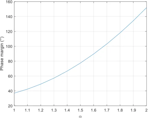
The obtained phase margin and gain crossover frequency as function of the fractional order is plotted in Figures1and2. For simplicity reasons is consideredT =TP= 1, without affecting the conclusions.
Mathematics 2019, 7, x FOR PEER REVIEW 7 of 24
Figure 1. Variation of phase margin with respect to the fractional order α.
Figure 2. Variation of gain crossover frequency with respect to the fractional order α.
Figure 1.Variation of phase margin with respect to the fractional orderα.
Mathematics 2019, 7, x FOR PEER REVIEW 7 of 24
Figure 1. Variation of phase margin with respect to the fractional order α.
Figure 2. Variation of gain crossover frequency with respect to the fractional order α.
Figure 2.Variation of gain crossover frequency with respect to the fractional orderα.
Mathematics2019,7, 1166 7 of 21
It can be observed that both gain crossover frequency and phase margin increases with the fractional orderα, meaning increased stability and smaller settling time as higher theαis. Forα=1 the “classical” Kessler’s phase margin value of 36.8◦and gain crossover frequency is obtained, as in Equation (10).
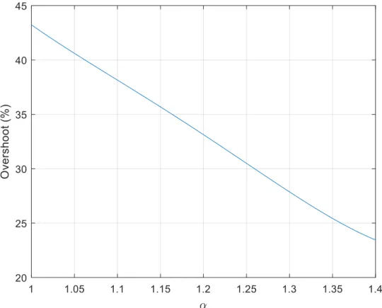
From the step response of the closed control loop with different values ofαthe corresponding overshoots can be determined, resulting the plot from Figure3. This plot reveals that the overshoot decreases with the increasing fractional order.
Mathematics 2019, 7, x FOR PEER REVIEW 8 of 24
Figure 3. Overshoot variation with respect to the fractional order α.
The main advantage of the Kessler’s optimum method-the steady state speed error cancellation-is maintained with the fractional order system as well. Moreover, the higher the fractional order, the better the transient response of the closed loop system, as it is presented in Figure 4.
Figure 3.Overshoot variation with respect to the fractional orderα.
The main advantage of the Kessler’s optimum method-the steady state speed error cancellation-is maintained with the fractional order system as well. Moreover, the higher the fractional order, the better the transient response of the closed loop system, as it is presented in Figure4.
Mathematics2019,7, 1166 8 of 21
Mathematics 2019, 7, x FOR PEER REVIEW 9 of 24
Figure 4. Transient for ramp input for different fractional order.
Having two more degrees of freedom-due to the parameter β and fractional order α–the controller design problem becomes an optimization problem: select the proper β and α to ensure the desired closed loop performance measures.
In Figure 5 the gain crossover frequency evolution (which is inversely proportional with the settling time) with respect to parameters β and α is presented. In a similar manner the maximum phase margin, Figure 6, or any other desired performance measure of the closed loop system can be represented. With this optimization technique the desired performances of the system can be ensured, no matter how rigorous they are.
Figure 4.Transient for ramp input for different fractional order.
Having two more degrees of freedom-due to the parameterβand fractional orderα–the controller design problem becomes an optimization problem: select the properβandαto ensure the desired closed loop performance measures.
In Figure5the gain crossover frequency evolution (which is inversely proportional with the settling time) with respect to parametersβandαis presented. In a similar manner the maximum phase margin, Figure6, or any other desired performance measure of the closed loop system can be represented. With this optimization technique the desired performances of the system can be ensured, no matter how rigorous they are.
Mathematics 2019, 7, x FOR PEER REVIEW 10 of 24
Figure 5. Gain crossover frequency evolution with respect to parameters β and α.
Figure 6. Phase margin evolution with respect to parameters β and α.
The controller parameter tuning algorithm can be described as follows:
Figure 5.Gain crossover frequency evolution with respect to parametersβandα.
Mathematics2019,7, 1166 9 of 21
Mathematics 2019, 7, x FOR PEER REVIEW 10 of 24
Figure 5. Gain crossover frequency evolution with respect to parameters β and α.
Figure 6. Phase margin evolution with respect to parameters β and α.
The controller parameter tuning algorithm can be described as follows:
Figure 6.Phase margin evolution with respect to parametersβandα.
The controller parameter tuning algorithm can be described as follows:
1. Having the process mathematical model of the form of Equation (5), the open loop transfer function form is imposed as in Equation (16) to provide zero steady-state position and velocity error.
2. Using Equations (18) and (19) the tuning parametersK,αandβfor the desired values of gain crossover frequency and phase margin are computed.
3. Having the open loop in Equation (17) and the process model in Equation (5), the transfer function of the fractional order controller in one of the forms presented in [22] is obtained.
The controller obtained with the proposed method being a fractional order one, engineers are faced with the problem of implementation. Actually, the fractional-order controller itself is an infinite-dimensional linear filter due to the fractional-order differentiator. A band-limit implementation is important in practice. Finite dimensional approximation of the fractional order controller should be used in a proper range of frequency of practical interest. A possible approximation method, the most widely applicable, is the Oustaloup recursive algorithm [23].
3. Case Studies
The results obtained with the controller tuning method presented in the previous section are illustrated.
3.1. Integer Order Plant, without Zero
It is considered a plant described by the transfer function:
HP(s) = 1
s(Ts+1). withT= 1,
a typical process model from mechatronics. This model could be the transfer function from position to armature voltage in a DC motor. Applying the general tuning rules presented in the introductory section, results the following nonlinear inequalities system:
KP r
1+2Kiω−gcλcosπ·λ
2 +ω−gc2λ·Ki2= pReHP2+ImHP2, Kisinπ·λ
2
ωλcg+Kicosπ·λ
2
=tan
π−φm+arctan ImHP
ReHP
,
Mathematics2019,7, 1166 10 of 21
Ki·λ·ωλgc−1·sinπ·λ
2
K2i +2ωλgc·Ki·cosπ·λ
2
+ω2λgc =
ReP|ω=ω
gc· d
dωImP ω=ω
gc
−ImP|ω=ω
gc· d
dωReP ω=ω
gc
ReP2 ω=ω
gc+ImP2 ω=ω
gc
,
KP2·
ω2λ+2Ki·ωλ·cosπ·λ
2
+K2i
hωλ(ReP+KP) +KiKP·cosπ2·λi2+hωλ·ImP−KiKP·sinπ·λ
2
i2 ≤A2,ω≥ωT, ω2λ·
ReP2+ImP2
hωλ(ReP+KP) +KiKP·cosπ2·λi2+hωλ·ImP−KiKP·sinπ·λ
2
i2 ≤B2,ω≤ωS, whereKp,Ki, and λare the tuning parameters of the fractional PI controllerHC(s) = KP
1+Ki
sλ
. The resulted system can be solved by optimization routines or approximation methods. A possible solution for the present case study, obtained with the fmincon command in Matlab®(20192-academic use, MathWorks, Inc., Natick, MA, USA) isKp=0.97,Ki=0.1 andλ=2.245. With these parameters the gain crossover frequency is 0.6 (rad/s) and the phase margin is 60◦.
As opposed to this complex design, following the proposed method at least the same performances can be achieved using simple, user-friendly equations, more suitable for industrial applications.
The open loop structure in this case is:
Hol(s) = k
s2·β2sα+1
sα+1 , α∈ <. The parametersαandβcan be established using the equations:
ωgc = 1 β
!α1
andk= 1 β
!2+αα .
The maximum achievable phase margin results from Equation (19):
arctan
β2−1 tanαπ2 (β+1)2+βtan2απ2 .
The design problem consists now in an optimization between the desired performances: finding the proper values ofβandαto have maximum value of the phase margin, maximum value of gain crossover frequency. With the chosen values ofβandα, the controller structure results from the open loop and the process transfer function.
In Table1the frequency domain performance measures are presented (phase margin, gain crossover frequency) and the control system main performance measures for a unit step input (overshoot, rise time) for different values of the parametersαandβ.
Mathematics2019,7, 1166 11 of 21
Table 1.Performance measures for differentβandαvalues.
α
Gain Crossover Frequency (rad/s)
Phase Margin (◦)
Overshoot (%)
Rise Time (s)
β=2
1 0.50 36.87 43.2 2.15
1.1 0.53 42.63 38.2 2.01
1.2 0.56 49.29 33.0 1.95
1.3 0.58 57.08 28.0 1.79
1.4 0.60 66.38 23.4 1.69
1.5 0.63 77.65 22.4 1.59
β=3
1 0.33 50.90 24.9 3.39
1.1 0.36 58.00 18.5 3.26
1.2 0.40 65.85 15.4 3.19
1.3 0.42 74.62 15.0 2.62
1.4 0.45 84.50 14.9 2.43
1.5 0.48 95.76 14.8 2.22
β=4
1 0.25 56.30 17.3 4.91
1.1 0.28 63.64 14.5 4.70
1.2 0.31 71.59 13.3 4.58
1.3 0.34 80.31 13.1 4.08
1.4 0.37 89.96 13.0 3.74
1.5 0.39 100.78 12.9 3.35
Figure7highlights the closed loop performance improvement for different fractional order in comparison with the Kessler’s optimum method values (α=1,β=2), while Figure8deals with the frequency domain measures. These simulation results are obtained using a second order “crone”
approximation of the fractional order in the frequency domain (10−2, 102) rad/s [23,24].
Mathematics 2019, 7, x FOR PEER REVIEW 13 of 24
Figure 7 highlights the closed loop performance improvement for different fractional order in comparison with the Kessler’s optimum method values (α = 1, β = 2), while Figure 8 deals with the frequency domain measures. These simulation results are obtained using a second order “crone”
approximation of the fractional order in the frequency domain (10 −2 , 10 2 ) rad/s [23,24].
Figure 7. Step response of the closed loop with integer order plant for different fractional order α and β = 2.
Figure 7.Step response of the closed loop with integer order plant for different fractional orderαand β=2.
Mathematics2019,7, 1166 12 of 21
Mathematics 2019, 7, x FOR PEER REVIEW 14 of 24
Figure 8. Bode plot of the control loop with integer order plant for different fractional order α and β = 2.
Comparing the results with the Kessler’s performance measures—indicated in the first row of the table, obtained for 1 , 2 , and with the blue line on Figures 7 and 8—the advantages are obvious. For example for 2 and 1 . 5 the achieved phase margin value is 77.65°, instead of 36.87° with the classical method, the overshoot is 22.4% instead of 43.2%, while the rise time is 1.59 s instead of 2.15 s. The integer order approximation of the designed controller is:
2
2 2
0.1071 0.3966 0.161 0.79311 9.961 1.461
( ) .
9.844 0.1016 1.113 1 9.844 0.1016 1.113 1
C
s s s
s s
H s
s s s s s s s s s s
For 4 and 1 . 5 a phase margin of 100.78°, overshoot 12.9% is obtained, but the rise time increases to 3.35 s. The best solution for the controller parameters can be achieved by an optimization procedure based on the imposed performance values.
3.2. Integer Order Plant with Zero
Another advantage of the method consists in the possibility to apply for a large variety of process models. For a process model having a zero, which is typical for parallel connected systems, the following transfer function is considered:
0.5 1 1 .
P
H s s
s s
The obtained performances are: for 1 . 3 and 2 the overshoot is 26.9%, rise time 1.74 s, phase margin 55.5°, gain crossover frequency 0.587 rad/s, while for 1 . 3 and 4 the overshoot decreases to 15.9%, phase margin increases to 83°, but the gain crossover frequency became 0.345 rad/s yielding a rise time of 4.23 s. These results are depicted in Figures 9–12.
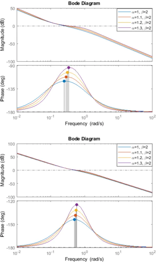
Figure 8.Bode plot of the control loop with integer order plant for different fractional orderαandβ=2.
Comparing the results with the Kessler’s performance measures—indicated in the first row of the table, obtained forα=1,β=2, and with the blue line on Figures7and8—the advantages are obvious.
For example forβ=2 andα=1.5 the achieved phase margin value is 77.65◦, instead of 36.87◦with the classical method, the overshoot is 22.4% instead of 43.2%, while the rise time is 1.59 s instead of 2.15 s. The integer order approximation of the designed controller is:
HC(s) = 0.79311(s+9.961)(s+1.461)
s(s+9.844)(s+0.1016)(s2+1.113s+1)+ (s+0.1071)s2+0.3966s+0.161 s(s+9.844)(s+0.1016)(s2+1.113s+1). Forβ=4 andα=1.5 a phase margin of 100.78◦, overshoot 12.9% is obtained, but the rise time increases to 3.35 s. The best solution for the controller parameters can be achieved by an optimization procedure based on the imposed performance values.
3.2. Integer Order Plant with Zero
Another advantage of the method consists in the possibility to apply for a large variety of process models. For a process model having a zero, which is typical for parallel connected systems, the following transfer function is considered:
HP(s) = 0.5s+1 s(s+1).
The obtained performances are: forα=1.3 andβ=2 the overshoot is 26.9%, rise time 1.74 s, phase margin 55.5◦, gain crossover frequency 0.587 rad/s, while forα=1.3 andβ=4 the overshoot decreases to 15.9%, phase margin increases to 83◦, but the gain crossover frequency became 0.345 rad/s yielding a rise time of 4.23 s. These results are depicted in Figures9–12.
Mathematics2019,7, 1166 13 of 21
Mathematics 2019, 7, x FOR PEER REVIEW 15 of 24
Figure 9. Step response of the closed loop with integer order plant with zero for different fractional order α and β = 2.
Figure 9.Step response of the closed loop with integer order plant with zero for different fractional orderαandβ=2.
MathematicsMathematics 2019, 7, 1166 2019,7, 1166 16 of 23 14 of 21
Figure 10. Bode plot of the control loop with integer order plant with zero for different fractional order α and β = 2.
Figure 10.Bode plot of the control loop with integer order plant with zero for different fractional order αandβ=2.
MathematicsMathematics 2019, 7, 1166 2019,7, 1166 17 of 23 15 of 21
Figure 11. Step response of the closed loop with integer order plant with zero for different fractional order α and β = 4.
Figure 12. Bode plot of the control loop with integer order plant with zero for different fractional order α and β = 4.
Figure 11.Step response of the closed loop with integer order plant with zero for different fractional orderαandβ=4.
Mathematics 2019, 7, 1166 17 of 23
Figure 11. Step response of the closed loop with integer order plant with zero for different fractional order α and β = 4.
Figure 12. Bode plot of the control loop with integer order plant with zero for different fractional order α and β = 4.
Figure 12.Bode plot of the control loop with integer order plant with zero for different fractional order αandβ=4.
Mathematics2019,7, 1166 16 of 21
The integer order approximation of the designed controller forα=1.3 andβ=2, the considered optimum in this case, is:
HC(s) = 0.94585(s+12.1)(s+1.881)
s(s+11.83)(s+2)(s+0.08454)(s2+1.729s+1)+ (s+0.2315)(s2+0.1845s+0.01243)
s(s+11.83)(s+2)(s+0.08454)(s2+1.729s+1). 3.3. Fractional Order Plant
The more general case considered is a fractional order plant. Such a process model is typical for effective modeling of high order control plants, for example of modeling experimental heat plant.
For:
HP(s) = 1 s1.5(s+1)
is consideredβ=2 andα=1.2 in the proposed algorithm. The obtained performances are: overshoot 33%, rise time 1.74 s, phase margin 48◦, gain crossover frequency 0.561 rad/s, while forα=1.2 and β=4 the overshoot decreases to 15%, phase margin increases to 67.9◦, but the gain crossover frequency became 0.315 rad/s yielding a rise time of 4.05 s. The steady-state velocity error is zero, as it is expected.
All these results are highlighted in Figures13–16. The integer order approximation of the designed controller in this case is:
HC(s) = B(s) A(s), where:
B(s) =793.1058(s+10)(s+9.961)(s+1.585)(s+1.461)
·(s+0.2512)(s+0.1071)(s+0.03981)(s+0.00631)s2+0.3966s+0.161 , A(s) =s(s+158.5)(s+25.12)(s+9.844)(s+3.981)
·(s+1)(s+0..631)(s+0.1016)(s+0.1)s2+1.113s+1 .
Mathematics 2019, 7, 1166 19 of 23
Figure 13. Step response of the closed loop with fractional order plant for different fractional order α and β = 2.
Figure 14. Bode plot of the control loop with fractional order plant for different fractional order α and β = 2.
Figure 13.Step response of the closed loop with fractional order plant for different fractional orderα andβ=2.
Mathematics2019,7, 1166 17 of 21
Mathematics 2019, 7, 1166 19 of 23
Figure 13. Step response of the closed loop with fractional order plant for different fractional order α and β = 2.
Figure 14. Bode plot of the control loop with fractional order plant for different fractional order α and β = 2.
Figure 14.Bode plot of the control loop with fractional order plant for different fractional orderαand β=2.
Mathematics 2019, 7, 1166 20 of 23
Figure 15. Step response of the closed loop with fractional order plant for different fractional order α and β = 4.
Figure 16. Bode plot of the control loop with fractional order plant for different fractional order α and β = 4.
Figure 15.Step response of the closed loop with fractional order plant for different fractional orderα andβ=4.
Mathematics2019,7, 1166 18 of 21
Mathematics 2019, 7, 1166 20 of 23
Figure 15. Step response of the closed loop with fractional order plant for different fractional order α and β = 4.
Figure 16. Bode plot of the control loop with fractional order plant for different fractional order α and β = 4.
Figure 16.Bode plot of the control loop with fractional order plant for different fractional orderαand β=4.
The cost of such a good results is the implementation of a fractional order controller, instead of a simple PI or PID controller, but with the present hardware possibilities this is not a real problem.
3.4. Experimental Case Study
In order to prove the efficiency of the proposed method, an experimental case study is included.
The DC motor is a versatile execution element which requires a certain degree of robustness due to varying operation conditions, load changes and other varying variables linked to it, making it a linear parameter varying system. It is explicitly chosen this example due to its simplicity in dynamics and operation. The experimental unit consists in the modular servo system designed by Inteco [25] used in the particular configuration indicated in Figure17. The plant is composed of a tachogenerator (used to measure the rotational speed), inertia load, backlash, incremental encoder, and gearbox with output disk.
Mathematics 2019, 7, 1166 21 of 23
The cost of such a good results is the implementation of a fractional order controller, instead of a simple PI or PID controller, but with the present hardware possibilities this is not a real problem.
3.4. Experimental Case Study
In order to prove the efficiency of the proposed method, an experimental case study is included.
The DC motor is a versatile execution element which requires a certain degree of robustness due to varying operation conditions, load changes and other varying variables linked to it, making it a linear parameter varying system. It is explicitly chosen this example due to its simplicity in dynamics and operation. The experimental unit consists in the modular servo system designed by Inteco [25] used in the particular configuration indicated in Figure 17. The plant is composed of a tachogenerator (used to measure the rotational speed), inertia load, backlash, incremental encoder, and gearbox with output disk.
Figure 17. The experimental unit: the modular servo system.
The mathematical model of the modular servo system without backlash and loads has been determined experimentally for the operating point of 100 rad/s as:
( ) ( )
( )
( 1) (0.6194 1),P
s k
H s u s s Ts s s
=Ω = =
+ +
where Ω is the angular position of the rotor and u is the input voltage.
Applying the proposed method, it is imposed:
2 2
( ) 1.
ol 1
k Ts H s s Ts
α α
β +
= ⋅ +
For a gain crossover frequency ωgc = 0.75 and phase margin PM = 72°, using Equations (19) and (20), the parameters α = 1.5, β = 2 and k = 0.198 are obtained. Computing the controller transfer function from
the well-known equation ( )
( ) ( )
ol C
P
H s H s
= H s results
( ) ( )
( )
1.5 1.5
2.4 1 0.6 1
( ) 0.001
0.6 1
C
s s
H s s s
+ +
= ⋅
+ .
Approximating this fractional order transfer function with the Oustaloup recursive approximation, results:
5 4 3 2
5 4 3 4
0.793 9.459 16.270 7.672 2.505 0.199
( ) .
11.060 13.070 11.060
C
s s s s s
H s s s s s s
+ + + + +
= + + + +
Figure 17.The experimental unit: the modular servo system.
Mathematics2019,7, 1166 19 of 21
The mathematical model of the modular servo system without backlash and loads has been determined experimentally for the operating point of 100 rad/s as:
HP(s) = Ω(s)
u(s) = k
s(Ts+1) = 194 s(0.6s+1), whereΩis the angular position of the rotor anduis the input voltage.
Applying the proposed method, it is imposed:
Hol(s) = k
s2·β2Tsα+1 Tsα+1 .
For a gain crossover frequencyωgc=0.75 and phase margin PM=72◦, using Equations (19) and (20), the parametersα=1.5,β=2 andk=0.198 are obtained. Computing the controller transfer function from the well-known equationHC(s) = HHol(s)
P(s) resultsHC(s) =0.001·(2.4s1.5+1)(0.6s+1)
s(0.6s1.5+1) . Approximating this fractional order transfer function with the Oustaloup recursive approximation, results:
HC(s) = 0.793s
5+9.459s4+16.270s3+7.672s2+2.505s+0.199 s5+11.060s4+13.070s3+11.060s4+s .
This controller was implemented using a specialized RT-DAC/PCI-D I/O board and the Real Time Windows Target toolbox from Matlab®. The obtained results are in accordance with the imposed values, as it is presented in Figure18.
Mathematics 2019, 7, x FOR PEER REVIEW 22 of 24
This controller was implemented using a specialized RT-DAC/PCI-D I/O board and the Real Time Windows Target toolbox from Matlab®. The obtained results are in accordance with the imposed values, as it is presented in Figure 18.
Figure 18. Response of the DC motor for a square input signal.
4. Conclusions
A novel tuning method for fractional order controllers is presented, inspired by the Kessler’s optimum method. The major advantages of the method are:
1. Ensures practically any closed loop performance measures, given the possibility to choose the most convenient solution by optimization for the tuning parameters α and β. Each solution will ensure the maximum possible value of the phase margin.
2. It is a simple method of the same complexity as the Kessler’s optimum method.
3. It can be applied for practically any type of process model, from integer order models to fractional order models, which can be approximated as in Equation (9).
All the main points of this work were verified both by numerical simulation and experimental results. The simulated case studies include process transfer functions with integer order, with zeros and fractional order transfer functions as well. As an experimental case study it was chosen as an example of great simplicity in mechatronic applications and basic loop control in the manifold of production systems: the DC motor.
Funding: This research was funded by Hungarian Academy of Science, Janos Bolyai Grant (BO/ 00313/17) and Bolyai+ Grant (Ú NKP-19-4-OE-64).
Conflicts of Interest: The author declares no conflict of interest.
Figure 18.Response of the DC motor for a square input signal.
4. Conclusions
A novel tuning method for fractional order controllers is presented, inspired by the Kessler’s optimum method. The major advantages of the method are:
Mathematics2019,7, 1166 20 of 21
1. Ensures practically any closed loop performance measures, given the possibility to choose the most convenient solution by optimization for the tuning parametersαandβ. Each solution will ensure the maximum possible value of the phase margin.
2. It is a simple method of the same complexity as the Kessler’s optimum method.
3. It can be applied for practically any type of process model, from integer order models to fractional order models, which can be approximated as in Equation (9).
All the main points of this work were verified both by numerical simulation and experimental results. The simulated case studies include process transfer functions with integer order, with zeros and fractional order transfer functions as well. As an experimental case study it was chosen as an example of great simplicity in mechatronic applications and basic loop control in the manifold of production systems: the DC motor.
Funding:This research was funded by Hungarian Academy of Science, Janos Bolyai Grant (BO/00313/17) and Bolyai+Grant (ÚNKP-19-4-OE-64).
Acknowledgments: This research was supported by Hungaryan Academy of Science, Janos Bolyai Grant and theÚNKP-19-4-OE-64 NEW NATIONAL EXCELLENCE PROGRAM OF THE MINISTRY FOR INNOVATION AND TECHNOLOGY.
Conflicts of Interest:The author declares no conflict of interest.
References
1. Chen, Y.Q.; Petras, I.; Xue, D. Fractional order control-A tutorial. In Proceedings of the 2009 American Control Conference, St. Louis, MO, USA, 10–12 June 2009; pp. 1397–1411.
2. Tejado, I.; Vinagre, B.M.; Traver, J.E.; Prieto-Arranz, J.; Nuevo-Gallardo, C. Back to Basics: Meaning of the Parameters of Fractional Order PID Controllers.Mathematics2019,7, 530. [CrossRef]
3. Petráš, I.; Terpák, J. Fractional Calculus as a Simple Tool for Modeling and Analysis of Long Memory Process in Industry.Mathematics2019,7, 511. [CrossRef]
4. Gutiérrez, R.E.; Rosário, J.M.; Machado, J.T. Fractional Order Calculus: Basic Concepts and Engineering Applications.Math. Probl. Eng.2010,2010, 375858. [CrossRef]
5. Fathalla, A.R. Numerical Modeling of Fractional-Order Biological Systems.Abstr. Appl. Anal.2013,2013, 816803. [CrossRef]
6. Hilfer, R.Applications of Fractional Calculus in Physics; World Scientific: Singapore, Singapore, 2000. [CrossRef]
7. Miller, K.S.; Ross, B.An Introduction to the Fractional Calculus and Fractional Differential Equations; John Wiley &
Sons: New York, NY, USA, 1993.
8. Podlubny, I. Fractional-order systems and PIλDµ-controllers.IEEE Trans. Autom. Control.1999,44, 208–213.
[CrossRef]
9. Oustaloup, A.La Commande CRONE; Editions HERMES: Paris, France, 1991.
10. Bruzzone, L.; Fanghella, P. Fractional-Order Control of a Micrometric Linear Axis.J. Control. Sci. Eng.2013, 2013, 947428. [CrossRef]
11. Bruzzone, L.; Fanghella, P. Comparison of PDD1/2 and PDu Position Controls of a Second Order Linear System. In Proceedings of the 33rd IASTED International Conference on Modelling, Identification and Control MIC 2014, Innsbruck, Austria, 17–19 February 2014; pp. 182–188.
12. Monje, C.A.; Chen, Y.Q.; Vinagre, B.M.; Xue, D.; Feliu-Batlle, V.Fundamentals of Fractional-Order Systems;
Springer: London, UK, 2010.
13. Dulf, E.H.; Timis, D.; Muresan, C.I. Robust Fractional Order Controllers for Distributed Systems.
Acta Polytech. Hung.2017,14, 163–176.
14. Muresan, C.I.; Dulf, E.H.; Both, R. Vector-based tuning and experimental validation of fractional-order PI/PD controllers.Nonlinear Dyn.2016,84, 179–188. [CrossRef]
15. Padula, F.; Visioli, A. Tuning rules for optimal PID and fractional-order PID controllers.J. Process Control 2011,21, 69–81. [CrossRef]
16. Valerio, D.; da Costa, J.S. Tuning of fractional PID controllers with Ziegler Nichols-type rules.Signal Process.
2006,86, 2771–2784. [CrossRef]
Mathematics2019,7, 1166 21 of 21
17. Hmed, A.B.; Amairi, M.; Aoun, M.; Hamdi, S.E. Comparative study of some fractional PI controllers for first order plus time delay systems. In Proceedings of the 2017 18th International Conference on Sciences and Techniques of Automatic Control and Computer Engineering (STA), Monastir, Tunisia, 21–23 December 2017; pp. 278–283.
18. Garrappa, R.; Kaslik, E.; Popolizio, M. Evaluation of Fractional Integrals and Derivatives of Elementary Functions: Overview and Tutorial.Mathematics2019,7, 407. [CrossRef]
19. Kessler, C. Das symmetrische Optimum.Regelungstechnik1958,6, 432–436.
20. Voda, A.A.; Landau, I.D. A Method for the Auto-calibration of PID Controllers.Automatica1995,31, 41–53.
[CrossRef]
21. Preitl, S.; Precup, R.E. An extension of tuning relations after symmetrical optimum method for PI and PID controllers.Automatica1999,35, 1731–1736. [CrossRef]
22. Ahmadi Dastjerdi, A.; Vinagre, B.M.; Chen, Y.Q.; HosseinNia, S.H. Linear fractional order controllers;
A survey in the frequency domain.Annu. Rev. Control2019,47, 51–70. [CrossRef]
23. Oustaloup, A.; Levron, F.; Mathieu, B.; Nanot, F.M. Frequency-band complex noninteger differentiator:
Characterization and synthesis.IEEE Trans. Circuits Syst. I2000,47, 25–39. [CrossRef]
24. Oustaloup, A.; Sabatier, J.; Lanusse, P.; Malti, R.; Melchior, P.; Moreau, X.; Moze, M. An overview of the crone approach in system analysis, modeling and identification, observation and control. IFAC Proc. 2008,41, 14254–14265. [CrossRef]
25. Inteco, Poland. Modular Servo System-User’s Manual. Available online:www.inteco.com.pl(accessed on 26 August 2019).
©2019 by the author. Licensee MDPI, Basel, Switzerland. This article is an open access article distributed under the terms and conditions of the Creative Commons Attribution (CC BY) license (http://creativecommons.org/licenses/by/4.0/).