Position, Size and Orientation Estimation of Ground Obstacles in Sense and Avoid ?
Peter Bauer∗
∗Systems and Control Laboratory, Institute for Computer Science and Control, Hungarian Academy of Sciences, H-1111 Budapest Kende
utca 13-17., (e-mails: bauer.peter@sztaki.mta.hu).
Abstract: This article is the improvement of the author’s previous work which considered position and size estimation of steady ground obstacles applying disc projection model and a constant velocity straight trajectory assumption. In case of square objects (trucks, buildings) the disc projection model can be a very rough approximation and so its improvement is required.
This paper presents a method to estimate the orientation of the square object and applies a line projection model which gives more precise size and position estimates. The formulas of the previous work were also improved to consider non-constant velocity non-straight trajectories but extensively tested with only constant velocity and straight trajectory assumptions to first prove applicability in a simpler case.
Keywords:Obstacle detection, Ground obstacle, Position estimation, Size estimation 1. INTRODUCTION
Usually aircraft (A/C) sense and avoid (S&A) is under- stood as the sensing and avoidance of aerial vehicles, how- ever in case of low level flight with small UAVs the avoid- ance of ground obstacles - such as transmission towers, tower-cranes, smokestacks or even tall tress - can be also vital to integrate them into the airspace. During landing or in case of emergency landing the presence of ground vehicles and buildings can also be dangerous and should lead to a go-around or landing place modification. This means that a small UAV’s S&A system should be prepared also to detect and avoid ground obstacles. Considering the size, weight and power constraints a monocular vision- based solution can be cost and weight effective therefore especially good for small UAVs Mejias et al. (2016), Nuss- berger et al. (2016). Placing a vision system onboard can also help the obstacle avoidance and landing of manned aircraft as the EU-Japan H2020 research project VISION (2016) shows through its research goals.
In the literature, the detection and avoidance of ground obstacles is discussed for example in Kikutis et al. (2017), Esrafilian and Taghirad (2016) and Saunders et al. (2009).
An example of ground object size estimation can be found in Shahdib et al. (2013) applying monocular camera and
? This is the author version of article published at IFAC ACA 2019 Conference (IFAC).c This paper was supported by the J´anos Bolyai Research Scholarship of the Hungarian Academy of Sciences. The research presented in this paper was funded by the Higher Education Institutional Excellence Program. The research leading to these results has received funding from the European Union’s Horizon 2020 research and innovation programme under grant agreement No. 690811 and the Japan New Energy and Indus- trial Technology Development Organization under grant agreement No. 062600 as a part of the EU/Japan joint research project entitled
’Validation of Integrated Safety-enhanced Intelligent flight cONtrol (VISION)’.
ultrasonic sensor. Kikutis et al. (2017) discusses path plan- ning to avoid obstacles with known position. Esrafilian and Taghirad (2016) discusses monocular SLAM-based obsta- cle avoidance applying also an altitude sonar. Real flight test results are also presented with a quadrotor helicopter and applying ground station-based calculations. Saunders et al. (2009) proposes an obstacle range estimation solution based-on A/C velocity and the numerical differentiation of yaw angle and obstacle bearing angle. This solution can give uncertain results because of the numerical differenti- ation in case of noisy measurements. Another restriction is that a close to zero pitch angle is assumed.
Previous works of the author of this article Bauer et al.
(2016), Bauer et al. (2017), Bauer and Hiba (2017) focused on the S&A of aerial vehicles applying monocular camera system with onboard image processing and restricting A/C movement to constant velocity and straight trajectories.
This work was extended for steady ground obstacles in Bauer et al. (2018) without the need for numerical differ- entiation and assuming constant own velocity and straight flight trajectory. A disc projection obstacle geometrical model was used and promising results obtained for cylinder and car objects. The results for cylinder were better as the disc projection model well fits the cylinder geometry while the square car model is far from a cylinder. This motivates the first goal of this article, to better handle square objects. The second goal is to extend the formulas (both for disc and square objects) for time-varying velocity and non-straight trajectories and improve the precision of object height estimation. The present article finally derives formulas to determine the position and size of circular or square ground obstacles even in case of time-varying own velocity and non-straight trajectories. The developed methods are tested in software-in-the-loop (SIL) simula- tion for artificial cylinder, truck, long truck and building objects. The car model from Bauer et al. (2018) was proven
to be too small to successfully demonstrate the advantages of edge detection that’s why its missing from here.
The structure of the paper is as follows. Section 2 discusses the problem of square object projection and proposes a solution. Section 3 extends the previous solutions of the author to time-varying velocity and non-straight trajecto- ries. Section 4 introduces the SIL simulation and evaluates the test results. Finally, Section 5 concludes the paper.
2. PROJECTION OF SQUARE OBJECTS Before discussing the calculations it is required to define the coordinate systems. In Fig. 1XE, YE, ZE is the Earth (assumed to be fixed, non-moving, non-rotating), X, Y, Z is the trajectory (Z axis parallel with the straight tra- jectory (dotted line) and moves together with the A/C), XB, YB, ZB is the body (moves with trajectory system and rotates relative to it) and XC, YC, ZC is the camera coordinate system (with fixed position and orientation relative to the body system). Note that also in case of non-straight motion it is assumed that there is an intended flight direction which gives the trajectory system orienta- tion.
XC
YC
ZC
XB
YB
ZB
Z
Y X XE
YE
ZE
Fig. 1. The applied coordinate systems
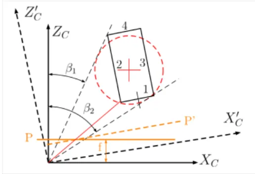
The disc projection model shown in Fig. 2 considers the tangents of the assumed disc in deriving the relations between object size and distance. However, this can lead to false size estimates if the projection of a rectangle is done as for example the projected size is a scaled combination of sides 1 and 2 in the figure.
Fig. 2. Projection of disc or rectangle
To obtain better results for square objects the projection of the line edges should be considered. However, this gives overly complicated formulas if the edge is not aligned with theXCaxis as discussed in Bauer et al. (2016). This means
that at first, the camera system should be aligned with the square object and then the line projection formulas can be applied. Determination of object orientation from the 2D image is discussed for example in Prematunga and Dharmaratne (2012) by considering a known size of the object and in Saxena et al. (2009) by applying learning algorithms. In our case the object size is unknown and our task is simpler then the one discussed in Saxena et al. (2009). By applying ego motion transformation of the image parameters from camera to body and then to trajectory system (for details see Bauer et al. (2018)) we can virtually align the camera with the trajectory system.
Assuming flat ground and that the object edges were detected its easy to determine object orientation relative to the trajectory considering the vanishing point along the trajectory ((0,0) image point in the aligned camera system). This is shown in Fig. 3. The edge of the object is parallel with cameraZC axis if it points into the (0,0) point. This gives the possibility to fit a line on the edges (1-2 and 2-3 in the figure) and determine its zero crossing (∆x distance) with XC. From this the required rotation angle (βC) to align the camera can be calculated (f is camera focal length):
y=a1x+a0, ∆x=−a1 a0
βC=atan
∆x
f
(1)
Of course, this alignment can only be done if the edges are not parallel withXC so this should be checked before.
Finally,βC can be used to virtually align the coordinate system by transforming the x coordinates of the image.
Fig. 3 shows the possible aligned edges with red dashed line and Fig. 2 shows camera system aligned with edge 1 (XC0 , ZC0 , P0).
Fig. 3. Camera alignment based-on vanishing point
After the virtual camera system alignment relations be- tween size and distances should be derived for the pro- jected line.
3. FORMULAS FOR TIME-VARYING VELOCITY AND NON-STRAIGHT TRAJECTORIES The formulas will be derived here both for the disc and the line projection models as they are very similar and all required in the test runs. The disc projection model for oblique cameras was derived in detail in Bauer et al.
(2017) resulting in:
Sx= ¯Sx(cosβ1+ cosβ2) =2f W ZC
x= ¯x
1− Sx2 16f2
=fXC ZC
(2)
Here, ¯Sx is the horizontal size of the disc image in the image plane (P), β1, β2 are the angles of the projected edges (see Fig. 2), ¯x is the horizontal position of the center of image, f is camera focal length, W is the real characteristic size of the object (disc model diameter) and XC, ZC are the real disc center positions in the camera system. In case of a line the projection formulas result as:
Sx=f W ZC
, x=fXC
ZC
(3) Here, Sx is the horizontal length of the line and xis the horizontal position of its center point in the image (see Fig. 2 edge 1). Considering the right hand sides formally only a 2 multiplier is the difference between disc and line projection. That’s why in the forthcoming, disc and line formulas will be unified with the multiplier in parenthesis.
Considering the βC real or virtual camera angle the XC, ZC camera system positions can be related to the trajectory system positions as follows:
XC=XcβC−ZsβC, ZC=ZcβC+XsβC (4) Where c and s stand for the cosine and sine functions respectively. In Bauer et al. (2018) theX, Zpositions were modeled by the assumed constant velocity of the A/C and time until reaching the object. In case of time-varying velocity and non-straight trajectories its better to model them as the difference of unknown initial distance and the distance flown by the A/C. So in a given time instant tk Xk = X0−∆Xk, Zk = Z0−∆Zk where ∆Xk,∆Zk
are assumed to be measurable by a GPS for example.
Substituting all these expressions into (2) and (3) results in the follwing system of equations attk:
(2)f
Sx(k) =sβC
X0
W +cβC
Z0
W −∆XksβC+ ∆ZkcβC
W (2)xk
Sx(k) =cβCX0
W −sβCZ0
W −∆XkcβC−∆ZksβC W
(5)
These are two equations with three constant unknowns X0/W, Z0/W and 1/W. Considering multiple time in- stants gives more equations and the possibility to solve the system. As a result the real W size (width) and the initial distances X0, Z0 can be obtained. From the latter its easy to obtain the actual distances asZk=Z0−∆Zk, Xk=X0−∆Xk.
In case of successful edge detection usually two edges of the object are visible. This gives the opportunity to determine also the L (length) size of the object by considering the projection of the other edge (see Fig. 3). Considering the coordinates of points 2,3 in the figure relative to the center of edge 1-2 gives the following formula:
S2= 1 x3 − 1
x2 = L
(XC−W/2)f (6) If one considers the other side of the rectangle then the sign of the W/2 term becomes positive. So finally the L size can be determined as:
Lk =S2(k)((X0−∆Xk)cβC−(Z0−∆Zk)sβC±W/2)f (7) This value can be calculated at each time when the terms on the right hand side are estimated. For better results a sliding window averaging can be applied.
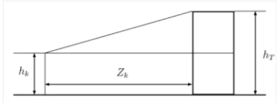
Finally, the vertical dimension should be handled by possi- bly determining the height of the obstacle. In Bauer et al.
(2018) a level flight was assumed and the aircraft rela- tive top point distance determined. Here, this method is modified assuming an altimeter and targeting to determine the ground relative height of obstacle top point to get acceptable results for descending or ascending trajectories also.
Fig. 4. Altitude estimation
Fig. 4 shows the concept of object altitude estimation.
Knowing the vertical coordinate of object top point from the image yT the absolute ground relative height can be determined attk as:
hT(k) =hk−yT(k)Zk
f (8)
Taking a moving average can decrease the variation of the estimated value.
4. SIL SIMULATION AND RESULTS
After developing the methods an extensive SIL test cam- paign was run to evaluate their performance similar to the one run in Bauer et al. (2018) but with different ground obstacles. A UAV following a straight trajectory with constant velocity (17m/s) (this is because at first, the formulas should be checked with the simplest case) was simulated in Matlab Simulink considering both A/C and autopilot dynamics. 0◦and 6◦glide slopes were considered.
A two camera system was modeled with 70◦horizontal and vertical field of view (FOV) of each camera and f = 914 but only the left camera was used placing all obstacles on the left side as formulas are symmetric so there is no need to test the right side also. Object projection was done applying pinhole camera model with pixelization error based-on point cloud in case of cylinder or the corners in case of other objects (modeled as cuboid) (see Table 1).
Image frequency was considered to be 8fps as this is the capability of state-of-the-art onboard hardware. Objects
were placed with different side distances and orientations (α = [−45, −20, 0, 20, 45] degrees relative to trajectory system) and different flight altitudes relative to object height were applied. Of course the cylinder is tested only with one orientation. The simulation run time (’run’ in Table) was set shorter then the time to reach the obstacle (’reach’ in Table) to be able to remain in camera FOV.
See Table 2 for all parameters. Note that for cylinder and building only half object height flight altitude was tested because with twice the object height altitude the object was out of camera FOV very early. All tests were run with both glide slope values (0◦/6◦).
The uncertainty in edge detection was modeled considering it only if the observed edge length was above 10 pixel.
Possibility to calculate object orientation was considered if the difference of vertical edge end point coordinates was larger then 2 pixels. Line projection model was considered only if both edge detection and orientation calculation were possible. Disc projection model was used before.
Solution of the system of equations (5) was done if 8 data points were collected. A moving window was applied after the first 8 data points. Disc equations were solved until the first 8 points were registered from the line model. For the square objects forced calculations using the disc model all the time were also run to be able to compare results with the proposed and theoretically more precise line model.
Table 1. Object parameters
Object W [m] L [m] H [m] Model
Cylinder 6 6 30 Point cloud
Building 15 40 89 Corners
Truck 2.5 7 2.5 Corners
Long truck 2.5 18 4 Corners
Table 2. Simulation parameters
Object X0 [m] H [m] Run [s] Reach [s]
Cylinder 0, 30, 60 15 19 20
Building 0, 75, 150 44.5 30 40
Truck 0, 12.5, 25 2.5, 5 18 20 Long truck 0, 12.5, 25 4, 8 18 20
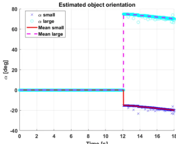
After running the tests detailed evaluation was done. Fig.
5 shows the convergence of the estimated orientation with building model and −20◦ real orientation. The estimates start close to the true values and converge to them. Also the larger angle of the other side is estimated and the estimates are smoothed by a low pass filter (Mean curves in the plot).
Fig. 5. Object orientation estimate
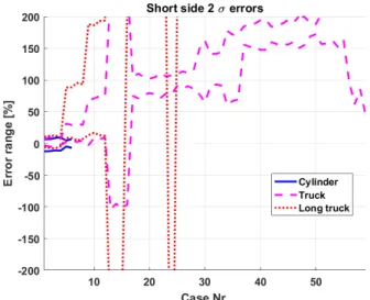
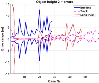
The 2σbounds of the percentage estimation errors for the Z0initial distance,X0side distance,W width andLlength are plotted in Fig.s 6 to 8 for the disc projection model and in Fig.s 9 to 12 for the line projection model (note thatL can not be determined by the disc projection so that figure is missing). The 2σbounds of the height estimation errors in meters are plotted in Fig.s 13 and 14 respectively. On the horizontal axes the case numbers show the number of simulations run with the given obstacle. The mean values were sorted into ascending order and then ±2σ added.
The results are summarized in Table 3. A simple number means that most of the values are inside that±range. A number with>means that most of the values are out of that range.
Table 3. Error statistics
Parameter: Z0 [%] X0[%] W [%] L [%] H [m]
Cylinder/disc 3 10 12 N/A 1
Truck/disc 5 >20 >50 N/A 2
Long truck/disc 5 >20 >50 N/A 2
Building/line 10 30 5 30 8
Truck/line 7 20 2 25 2
Long truck/line 7 25 2 25 2
Table 3 shows that in estimating the initial distance the disc model is a bit better than the line model even for the square objects while in the height estimation it performs equally well with the line model. Considering the side distance the line model is better for the square objects as the disc model is well outside the±20% range in most of the cases (see Fig. 7). The width estimation results are much more better with the line model then with the disc while length estimation results are more uncertain with as large as 25−30% error. Considering (7) this is not surprising as the calculation ofLcumulates all of the other estimation errors. Possibly the 25−30%X0error appears inLalso.
As a conclusion it can be stated that the disc projection model is applicable to determine the initial distance and height of both circular and square objects but it gives too large errors in side distance and size information for square objects, so its better to use the line model for them.
5. CONCLUSION
This paper presents the derivation of square object ori- entation estimation and a line projection model to better estimate the position and size of square objects considering a monocular camera in aircraft ground obstacle detec- tion. It also extends the previous results for time-varying velocity and non-straight trajectories both for disc and line object models. After deriving the formulas it runs a SIL simulation campaign in Matlab Simulink considering real aircraft dynamics with constant velocity and straight trajectory to evaluate their ideal performance. Cylinder, building, truck and long truck obstacles are considered.
The line projection performs much better in estimating the size and side position of the square objects so it is advisable to apply this new method if the edges of the detected objects can be determined. Future research will include detailed evaluation of the conditioning of system of equations as there were some outliers in the results and the test for time-varying velocity and non-straight trajectories considering also own position uncertainty.
Fig. 6. Initial distance (Z0) errors, disc model
Fig. 7. Side distance (X0) errors, disc model
Fig. 8. Short side (W) errors, disc model
Fig. 9. Initial distance (Z0) errors, line model
Fig. 10. Side distance (X0) errors, line model
Fig. 11. Short side (W) errors, line model
Fig. 12. Long side (L) errors, line model
Fig. 13. Height errors, disc model
Fig. 14. Height errors, line model
REFERENCES
Bauer, P., Hiba, A., Vanek, B., Zarandy, A., and Bokor, J.
(2016). Monocular Image-based Time to Collision and Closest Point of Approach Estimation. In In proceed- ings of 24th Mediterranean Conference on Control and Automation (MED’16). Athens, Greece.
Bauer, P. and Hiba, A. (2017). Vision Only Collision De- tection with Omnidirectional Multi-Camera System. In in Proc. of the 20th World Congress of the International Federation of Automatic Control, 15780–15785. IFAC, Toulouse, France.
Bauer, P., Hiba, A., and Bokor, J. (2017). Monocular Image-based Intruder Direction Estimation at Closest Point of Approach. In in Proc. of the International Conference on Unmanned Aircraft Systems (ICUAS) 2017, 1108–1117. ICUAS Association, Miami, FL, USA.
Bauer, P., Vanek, B., and Bokor, J. (2018). Monocular Vision-based Aircraft Ground Obstacle Classification.
InIn Proc. of European Control Conference 2018 (ECC 2018), 1827–1832.
Esrafilian, O. and Taghirad, H.D. (2016). Autonomous flight and obstacle avoidance of a quadrotor by monoc- ular slam. In 2016 4th International Conference on Robotics and Mechatronics (ICROM), 240–245. doi:
10.1109/ICRoM.2016.7886853.
Kikutis, R., Stankunas, J., Rudinskas, D., and Masiulionis, T. (2017). Adaptation of Dubins Paths for UAV Ground Obstacle Avoidance When Using a Low Cost On-Board GNSS Sensor. Sensors, 17(10), 1–23.
Mejias, L., McFadyen, A., and Ford, J.J. (2016). Feature article: Sense and avoid technology developments at Queensland University of Technology. IEEE Aerospace and Electronic Systems Magazine, 31(7), 28–37. doi:
10.1109/MAES.2016.150157.
Nussberger, A., Grabner, H., and Gool, L.V. (2016).
Feature article: Robust Aerial Object Tracking from an Airborne platform. IEEE Aerospace and Electronic Systems Magazine, 31(7), 38–46. doi:
10.1109/MAES.2016.150126.
Prematunga, H.G.L. and Dharmaratne, A.T. (2012). Find- ing 3D Positions from 2D Images Feasibility Analysis.
InIn Proc. of The Seventh International Conference on Systems (ICONS 2012).
Saunders, J., Beard, R., and Byrne, J. (2009). Vision- based reactive multiple obstacle avoidance for micro air vehicles. In 2009 American Control Conference, 5253–
5258. doi:10.1109/ACC.2009.5160535.
Saxena, A., Driemeyer, J., and Ng, A.Y. (2009). Learning 3-d object orientation from images. In 2009 IEEE International Conference on Robotics and Automation, 794–800. doi:10.1109/ROBOT.2009.5152855.
Shahdib, F., Wali Ullah Bhuiyan, M., Kamrul Hasan, M., and Mahmud, H. (2013). Obstacle detection and object size measurement for autonomous mobile robot using sensor.International Journal of Computer Applications, 66, 28–33. doi:10.5120/11114-6074.
VISION (2016). Vision project (validation of inte- grated safety-enhanced intelligent flight control). URL http://w3.onera.fr/h2020 vision/node/1.