Impacts of acid rain II.
Transmission in the air, the
transport of pollutant: a modeling approach
Lecture 15
Lessons 43-45
• Lesson 43
The Janus faced influence of regional level acid rains: local impacts are also included.
Different attacking points locally
Impacts of acid rain
• Although the acid rain has not stood center-stage
concerning today’s environmental problems, dramatic visions of corroding monuments and leafless trees may capture the public minds.
• Oppositely to other atmospheric hazards, the acid
deposition is the only event, that may be presented in different levels;
- the habitats are influenced locally, and at the same time
- regional lesions are also present.
The injuries may differ in form.
• Apparently, the treat of acid deposition has lost some of its actuality due to positive government policies and
results aimed to mitigate its impacts in the 1960s and
1970s. The problem is vital, mainly on some pointed out places of the world.
• There are two attacking points of the issue on ecosystem level
- The land ecosystems, the woods and the soil included - The water ecosystems
Local level means human health impacts and any other influences coming from the constituent of acid
deposition.
• It is important to see, that this atmospheric origin event has a twofold character; at the same time we should distinguish their short-term and long-term ecological effects. They are present simultaneously. The injuries separation may be carried out on academic level only!
The nature does not know about it.
• As a rule, the local influence as stress is mainly the impact of sulfur dioxide and nitric acid. In this situation the person, and a group of human beings or smaller units of crops and animals are suffer from impairment.
• The harm of acid rains may manifest even larger habitats; this coming from its regional point.
Touched areas in the world
• The acid deposition is present almost in all over the
world, but there are some places where the endangered area is more extended:
- A part of Europe including portions of Sweden, Norway, and Germany,
- the northeastern United States, - southeastern Canada,
- In addition, parts of North East Asia, South Africa, Sri Lanka, and Southern India.
Smaller „accidents” may happen on any other places of the world.
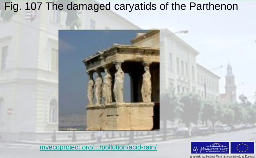
The acid rain was discovered by a Scottish chemist, Robert Angus Smith, in 1852. He was the first, who has written the connection between changed rainwater quality and negative events found in Manchester, England. Although it was discovered in the 1800s, acid rains did not get
significant attention until the heavy traffic of 1960s. The term itself was coined in 1972. There were some crucial aftermath such as the corrosion of the famous statues of Athen (caryatids), that pay public attention. In
environmental pollution the word of corrosion is applied wider, not only for metals; limestone buildings, papers, vehicles, tissues, etc.; anything above and below the ground.
Fig. 107 The damaged caryatids of the Parthenon
myecoproject.org/.../pollution/acid-rain/
Impacts on man-made environment
• Especially the limestone buildings and statues are
endangered because the acids react with minerals in the stones and it disintegrates and washes away.
• The ways of damaging the historical and other monuments are,
- Aqueous dissolution reactions of calcium carbonate.
Most susceptible are the limestone monuments.
- Some gaseous pollutants (SO2), may form of gypsum layer in surface crusts.
- Particle deposition on stone surfaces. These pollutants may catalyze processes to accentuate damage on the stone surface.
• A possible reaction of writing the change in limestone is CaCO3 +2HNO3 CO2 + Ca(NO3)2 + H2O.
We note, that the quartz is resistant to acids. Taking into account the above hints, the lesion of acid rain may be estimated as follows. Let’s take the limestone sample contains only calcite (c) and quartz (q), and its initial weight is mii
mii = m c + mq
After the acid rains the final weight (mf) will be:
mf= mn+ mq
where mndenotes the formed calcium nitrate weight.
Finally the destroyed limestone can get easily.
Effects on the human health
• In the past decades epidemiological studies presented relationship between the ambient fine particle
concentrations, among the others sulfates and nitrates formed in the atmosphere from SO2 and NOx emissions, and health problems. The high number of heart and lung disease, than the increased incidences of respiratory
disease and symptoms (asthma, bronchitis), and even premature death can be classed here.
• Results of recent research show that small particles in the air caused more than 350,000 premature deaths within the 25 countries of the European Union in 2000.
• Scientists suspect that aluminum, one of the toxic metals affected released in soils by acid deposition, is in close connection with increasing Alzheimer’s disease in
human beings.
• Following the detrimental effect of acid rains, the most endangered group among the others is the human
population. It has the ability of harming via - the atmosphere as well as
- the soil where the food is „grown”.
- Consuming the produced final products (crops,
animals) may be polluted. The humans stand on the top of pyramid!
• Lesson 44
Impacts on land ecosystems
Impacts on aquatic ecosystems
Land ecosystems - forests
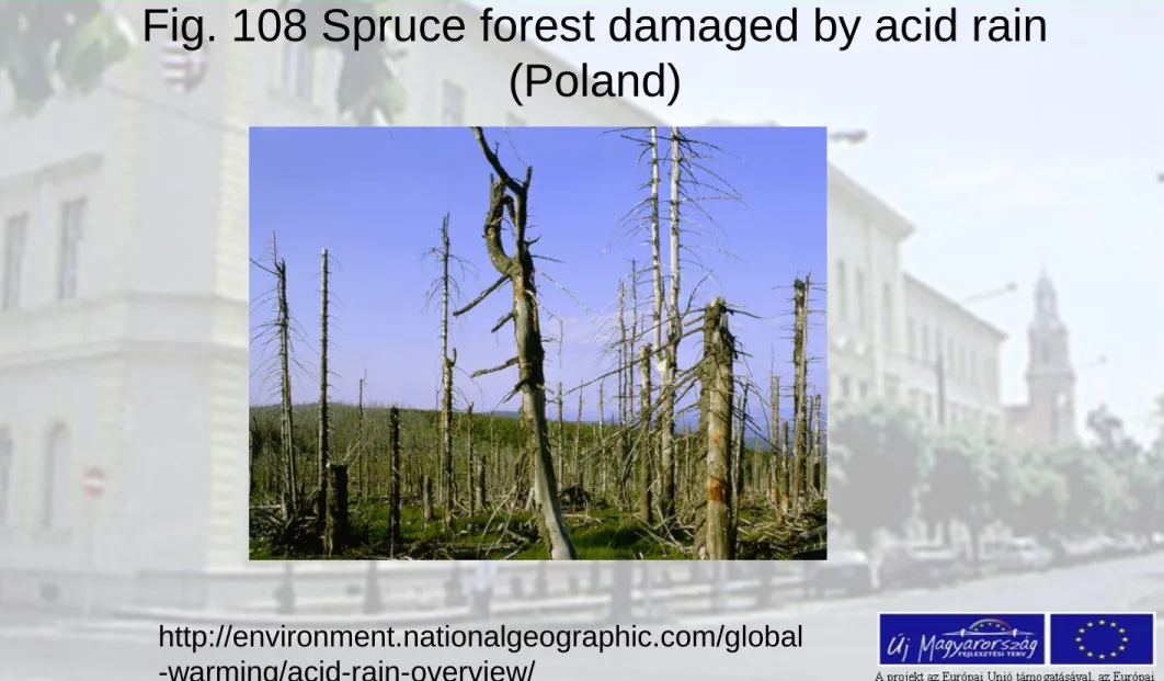
• Observations show that, individual trees or in some exceptional cases entire areas of the forest died off
without any „obvious” reason, during the past decades.
Even in summer the green leaves (needles) turn brown and fall off from the tree. As a result of early stop of
vegetation period, the growth of trees is slowing down.
• Until now we started to understand the difference in tolerance of acid rain between altered places. The soil buffering capacity determines basically the susceptibility of a given wood to acid deposition. The rain reaches the soil surface, and if the soil buffering capacity is high, it may protect the trees living on there.
Fig. 108 Spruce forest damaged by acid rain (Poland)
http://environment.nationalgeographic.com/global -warming/acid-rain-overview/
• The acid deposition acts through different classes:
- damaging the green leaves, destructing the chlorophyll content and photosynthesis
- limiting the soil nutrients availability
- exposing to toxic substances slowly released from the soil.
Finally the damage or death of trees is the combination of the above factors coming from acid rain. In some special cases only one threat may be enough to harm the
ecosystem. All the cited causes alone or in combination weaken the tree’s immune system. Other stress factors as drought may finish this started negative action.
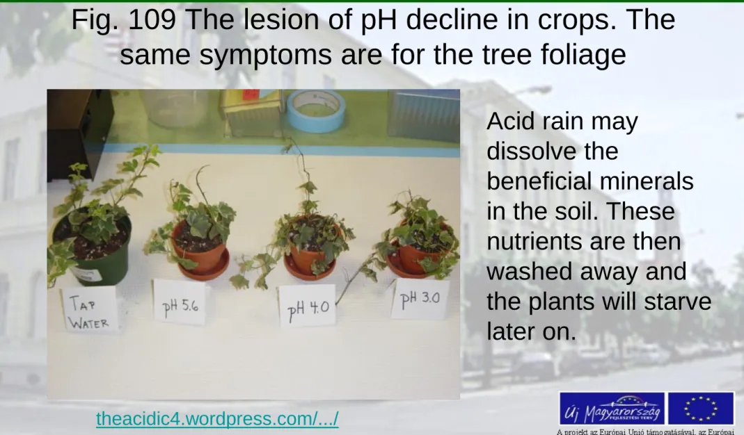
Fig. 109 The lesion of pH decline in crops. The same symptoms are for the tree foliage
theacidic4.wordpress.com/.../
Acid rain may dissolve the
beneficial minerals in the soil. These nutrients are then washed away and the plants will starve later on.
Aquatic ecosystems
• In general, the pH of the lakes and other streams is between 6 and 8, although there are a few of them
naturally acidic even without any environmental acidity.
These habitats are the most sensitive ones, highly
endangered by acid rains. The reason of the increased sensitivity roots in the bottom of the lakes; their basic soil layer has no or limited ability to neutralize acidic
compounds (granite bottom). The buffering capacity of this lake is low. In areas, where buffering capacity is limited, the acid rain releases aluminum from the
sediments into lake water. The aluminum is a very toxic heavy metal to species of aquatic and other habitats.
• There are some episodic acidification also referring to brief periods during which pH levels decline in mountain areas due to runoff from melting snow or heavy
downpours. The temporarily acidic used to appear during heavy storms and spring snowmelt. On a large scale the geographical position determines the risk of episodic
acidification. Episodic acidification may the reason of the so called “fish kills.”
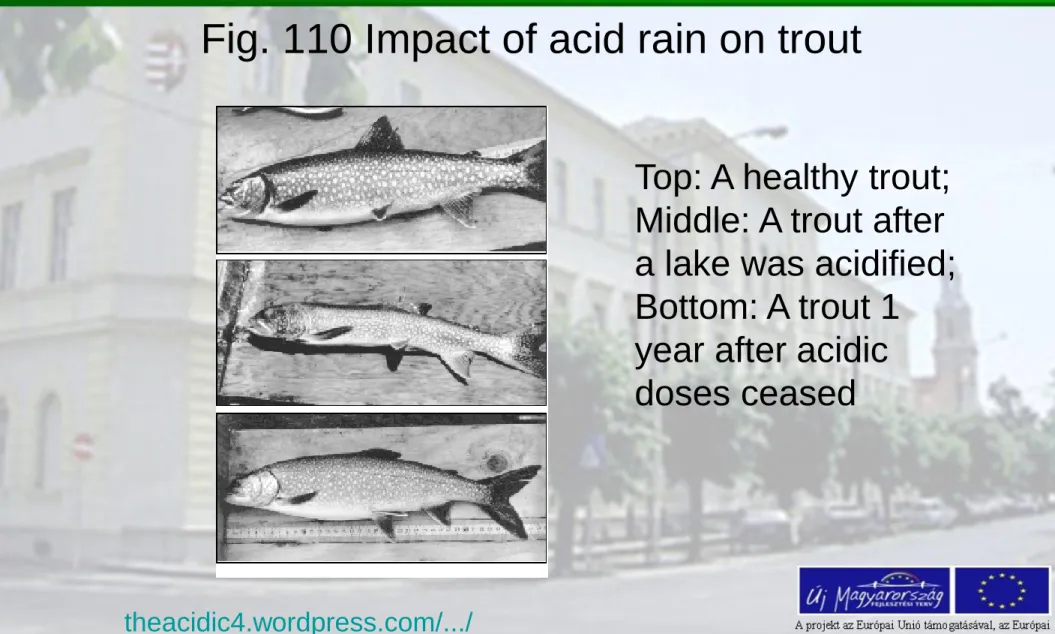
• Not only the released aluminum, but the pH decline also kills the living organisms. Probably the stress associated with the above factors impairs the fish. The stress does not kill them, but leads to lower body weight and smaller size.
Fig. 110 Impact of acid rain on trout
Top: A healthy trout;
Middle: A trout after a lake was acidified;
Bottom: A trout 1 year after acidic doses ceased
theacidic4.wordpress.com/.../
• The smaller size of fish deteriorates the chance in competition for foods and life struggle.
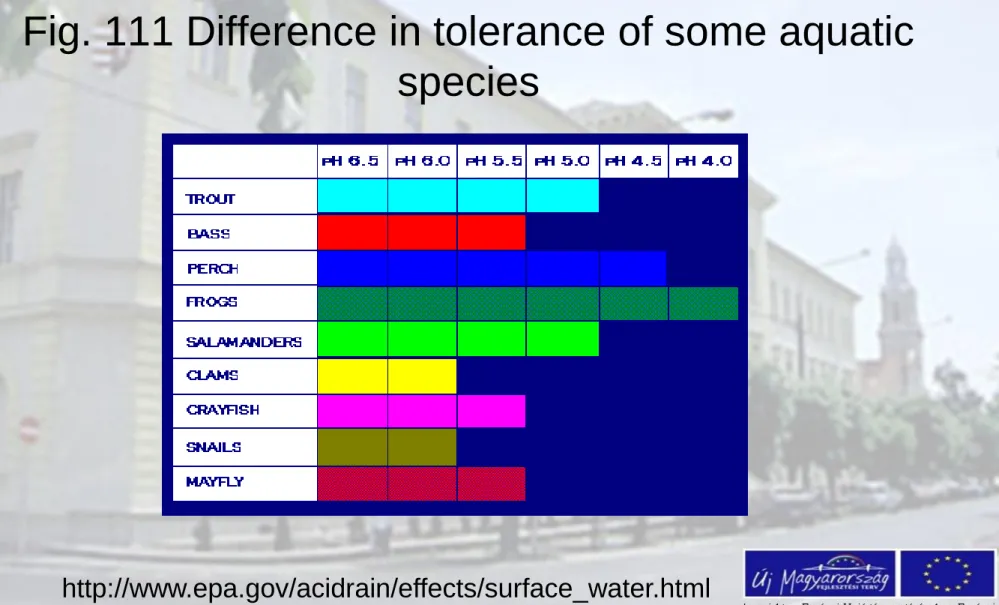
There are some tolerant plants and animal species.
Generally, the young ones of the most species are more sensitive to environmental conditions than adults.
- At pH 5, most fish eggs cannot hatch.
- At lower pH levels young fish may die.
- Below pH 3 there is no fish in the lake.
The next chart shows the difference in tolerance of animals living in water bodies. Frogs can tolerate polluted water that is more acidic i.e. than trout.
Fig. 111 Difference in tolerance of some aquatic species
http://www.epa.gov/acidrain/effects/surface_water.html
Strong interactions exist between the members of the ecosystems.
The frogs can tolerate relatively low pH values in the water, but if they eat susceptive insects as the mayfly, they
would also be harmed through their food supply (food chain). Not only the sensitive species among the others the mayfly, may cease.
This is not a very often mentioned example how the
extinction of species may happen outside the frequent cited global warming; in case of regional or local level acid deposition.
• Lesson 45
Modeling the transport of pollutant in the air Gaussian model
Euler model
Lagrange model
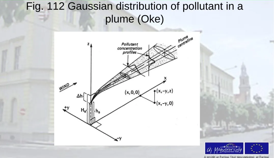
Pollutant transport in the air The Gaussian model
• The pollutant concentration in a plume is centered horizontally; the peak amount is in the plum centre. A
bell-shaped profile of trace concentration is formed in the vertical plane of the plume. The plume width is
continuously expanding and the concentration is descending in time.
• In Gaussian model the zero concentration is valid at the place of emission, then the concentration is rising until it reaches its peak, and later on it is falling. It is important, that the concentration is always the highest in the
centerline of the plume.
Fig. 112 Gaussian distribution of pollutant in a
plume (Oke)
• The Gaussian normal distribution has some random errors as well. Translating it, to evaluate the pollution distribution by applying the Gaussian curve means, that random atmospheric turbulence mixes the pollutants,
and their concentration is distributed normally around the central axis of the plume. The normal distribution is valid for both horizontal, y and vertical, z planes. This
assumption helps to evaluate the pollutant dispersion in the air of traces (small sized particle) on
- local pollution level,
- assuming continuous emission, and - taking into account the point sources .
• To calculate the contamination concentration for an x trace at any point within the plum the following equation is needed:
z y y z
y x
y u
x x
2 2 )
, ,
( 2
exp
2
z s z
s z H
H x z
2
2 2
2
2
) exp (
2
) exp (
• where denotations stands for
x – rate of emission at the source in kg s-1,
σy and σz - horizontal and vertical standard deviations of the pollutant in the directions of y and z [m],
u - average wind speed along the plum centre [m s-1], Hs – calculated effective stack height [m].
The result for pollutant concentration (mass concentration) then will be in kg m-3, or μg m-3.
The effective stack height, H s is the composition of real stack height (h s) and additional one (Δh) resulted from plum rise, see Fig. 104. The actual meteorological
conditions determine the value of plum rise.
The Euler model
• The most universal assumption in calculation the dispersion of traces is the Euler modeling. This
projection is applicable for every types of pollution; for local, regional and also for global ones.
• The model input comprises two components; the
horizontal air motion (TR) and the turbulent flux (TIR). If the axis x points on the direction of wind, then the
gradient of concentration, C and gradient of wind speed, u will be
x u
x C
and respectively.
Fig. 113 The sketch of the Euler model
a) Rendezett- Te
b) Függőleges- Tt
m
• The mass, m of the pollutant is the multiplication of the wind speed and concentration of the given contaminant.
The input of the model is the mass of traces (m = u C).
(Vertically, the turbulence also adds a portion to the contamination level.)
• Horizontal output of the model will be (see negative sign!)
From the two components of contaminant transport the horizontal change will be:
) ) ( (
x uC uC
The other type of air mass attenuation is the turbulence. K is the diffusion coefficient. The input side is:
The amount of pollutant mass leaving our „sample box”
with turbulence is
TRx
x uC t
C
( )
) (
x K x C
x K C
x x
K x C x
• The concentration change in the system then:
The complete concentration change for the given pollutant is the sum, Tx of the two concentration changes,
Tx = TRx + TIRx
Similarly to the presented x direction, we have to write the equations for the other two lacking coordinates (y,z) as well. Our example is for x only.
IRx
x T
x K C
x t
C
( )
• The actual concentration of pollutant depends on other factors as well. They may increase or decline the actual concentration level;
- The emission, S rises,
- Deposition, D declines, and
- Chemical transformations, FR may modify in both - negative or positive – directions of the actual pollutant concentration.
Taking into account all the influencing factors we get for the concentration change, C
FR D
S T
T t
C
IR
R
Lagrange or „box” model
• The sample box is moving with the air motion. The actual height of our sample box is equal to the height of the
mixing layer, H. Let us choose a unit surface area box for the easy treating of model input variables. The
concentration of the pollutant inside the box is
considered homogeneous. The box is closed from the top, and emission, Q, depositions (wet and dry) and chemical reactions determine the given pollutant
concentration. The turbulence is omitted in this type of approach.
• In this consideration we use more coefficients; k1,k2, and k3 stand for chemical reaction and dry and wet
depositions, respectively.
The k1 has to be measured in lab or in the field (for chemical transformation).
The k2 is calculated with knowing the dry deposition and mixing layer (H).
Finally k3 should be written as:
where ω – is the washing out ration P – is the precipitation.
dt dP H
k
3
The concentration change, C1 is:
where C1 is a pollutant, in most cases the primary one, for example the sulfur dioxide. This equation does not mean the end of our modeling, as the primary pollutant forms a secondary one, the C2. We have to follow the chemical reactions further. The concentration change for the
second trace (sulfate) is:
The k4 and k5 may similar to the earlier discussed coefficients.
2 5 2
4 1
1
2 k C k C k C
dt
dC
1 3 1
2 1
1
1 k C k C k C
H Q dt
dC