Time preferences and their life outcome correlates:

(1)

BUDAPEST WORKING PAPERS ON THE LABOUR MARKET

BWP – 2019/1

Time preferences and their life outcome correlates:

Evidence from a representative survey

DÁNIEL HORN – HUBERT JÁNOS KISS

BWP 2019/1

INSTITUTE OF ECONOMICS, CENTRE FOR ECONOMIC AND REGIONAL STUDIES HUNGARIAN ACADEMY OF SCIENCES

BUDAPEST, 2019

(2)

Budapest Working Papers on the Labour Market BWP – 2019/1

Institute of Economics, Centre for Economic and Regional Studies, Hungarian Academy of Sciences

Time preferences and their life outcome correlates:

Evidence from a representative survey

Authors:

Daniel Horn senior research fellow

Centre for Economic and Regional Studies, Hungarian Academy of Sciences, Hungary and Eötvös Loránd University

E-mail: horn.daniel@krtk.mta.hu

Hubert János Kiss senior research fellow

Centre for Economic and Regional Studies, Hungarian Academy of Sciences, Hungary and Eötvös Loránd University

E-mail: kiss.hubert.janos@krtk.mta.hu

February 2019

(3)

3 Time preferences and their life outcome correlates:

Evidence from a representative survey

Dániel Horn - Hubert János Kiss Abstract

We collect data on time preferences of a representative sample of the Hungarian population in a non-incentivized way and investigate how patience and present bias associate with important life outcomes in five domains: i) educational attainment, ii) unemployment, iii) income and wealth, iv) financial decisions and difficulties, and v) health. Based on the literature, we formulate the broad hypotheses that patience fosters, while present bias hinders positive outcomes in the domains under study. We document a consistent and often significant positive effect of patience in almost all areas (except unemployment), with the strongest effects in escaping low educational attainment, wealth and financial decisions. We find that present bias associates significantly with saving decisions and financial troubles.

Keywords: educational attainment, financial decisions and difficulties, income and wealth, patience, present bias, risk preferences.

JEL codes: D12, D14, D31, D90, I12, I21, J6

Acknowledgement:

We are very grateful to Péter Biró, László Halpern, Marc Kaufmann, Balázs Kertész,

László Lőrincz, Brigitta Németh and János Vince for enlightening comments, and thank

participants of research seminar at the Institute of Economics of the Hungarian

Academy of Sciences and the annual conference of the Hungarian Society of Economics

for their helpful comments. The usual disclaimers apply.

(4)

4 Mivel korrelálnak az időpreferenciák?

Egy reprezentatív felmérés eredményei

Horn Dániel – Kiss Hubert János

Összefoglaló

Egy magyar reprezentatív felmérés kereteiben mértük fel a válaszadók időpreferenciáit, nem ösztönzött módon. A kutatásban azt vizsgáljuk, hogy az időpreferencia egyes aspektusai – a türelem illetve a jelen-torzítottság – hogyan függnek össze különböző kimenetekkel az életút során. A tanulmányban azt vizsgáljuk, hogy az időpreferencia e két aspektusa hogyan függ össze az i) oktatási szinttel, ii) munkanélküliséggel, iii) jövedelemmel és vagyonnal, iv) pénzügyi döntésekkel és pénzügyi nehézségekkel, v) egészséggel. Az irodalom alapján azt feltételezzük, hogy a türelem pozitívan, míg a jelen- torzítottság negatívan függ össze a pozitív élet-kimenetekkel. Adataink alapján azt mondhatjuk, hogy a türelem szinte az összes vizsgált kimenettel (kivéve munkanélküliség) szignifikánsan és a várt irányban függ össze. A legszorosabb az összefüggés az alacsony iskolázottsággal, vagyonnal és a pénzügyi döntésekkel. A jelen- torzítottság összefüggései a kimenetekkel gyengébbek, de szignifikáns összefüggést találunk a megtakarítási döntések és a pénzügyi nehézségek esetében.

Tárgyszavak: oktatási szint, pénzügyi döntések, pénzügyi nehézségek, jövedelem, vagyon, türelem, jelen-torzítottság, kockázati preferenciák

JEL-kódok: D12, D14, D31, D90, I12, I21, J6

(5)

(will be inserted by the editor)

Time preferences and their life outcome correlates: Evidence from a representative survey

D´aniel Horn · Hubert J´anos Kiss

Abstract We collect data on time preferences of a representative sample of the Hungarian population in a non-incentivized way and investigate how patience and present bias associate with important life outcomes in five domains: i) educational attainment, ii) unemployment, iii) income and wealth, iv) financial decisions and difficulties, and v) health. Based on the literature, we formulate the broad hypotheses that patience fosters, while present bias hinders positive outcomes in the domains under study. We document a consistent and often significant positive effect of patience in almost all areas (except unemployment), with the strongest effects in escaping low educational attainment, wealth and financial decisions. We find that present bias associates significantly with saving decisions and financial troubles.

JEL classifications: D12, D14, D31, D90, I12, I21, J6.

Keywords: educational attainment, financial decisions and difficulties, income and wealth, patience, present bias, risk preferences.

We are very grateful to Péter Biró, László Halpern, Marc Kaufmann, Balázs Kertész, László L˝orincz, Brigitta Németh and János Vince for enlightening comments, and thank participants of research seminar at the Institute of Economics of the Hungarian Academy of Sciences and the annual conference of the Hungarian Society of Economics for their helpful comments. The usual disclaimers apply.

MTA KRTK KTI and Eötvös Loránd University

1097 Budapest, Tóth Kálmán u. 4. and 1117 Budapest, Pázmány sétány 1/a, Hungary.

E-mail: horn.daniel@krtk.mta.hu ORCID: 0000-0002-2888-6240

Financial support from the National Research, Development & Innovation (NKFIH) under project K 124396 is gratefully acknowledged.

MTA KRTK KTI and Eötvös Loránd University

1097 Budapest, Tóth Kálmán u. 4. and 1117 Budapest, Pázmány sétány 1/a, Hungary.

Tel.: +36-30-4938062

E-mail: kiss.hubert.janos@krtk.mta.hu ORCID: 0000-0003-3666-9331

Financial support from the Spanish Ministry of Economy, Industry and Competitiveness under the project ECO2017-82449-P, the Hungarian Scientific Research Fund (OTKA) under project 109354, the National Re- search, Development & Innovation (NKFIH) under project K 119683 is gratefully acknowledged.

(6)

1 Introduction

Economic analysis is based on the tenet that individuals maximize utility functions that are representations of preferences, given some constraints. One of the most basic preferences that appear in almost all introductory books on Economics aretime preferences. There are two relevant aspects of time preferences that we study in this paper. On the one hand, patience reveals how an individual values the future relative to the present, hence it plays an essential role in intertemporal decision-making. Importantly, patient individuals have a low discount rate, so they appreciate future benefits more than their more impatient peers. Thus, as the cost of effort generally materializes in the present, more patient individuals are expected to invest more today in things that bear fruits tomorrow. As a consequence, more patient individuals may tend

– to invest more in their human capital by studying more;

– to choose long-term financial investments (e.g. retirement savings);

– to lead a more healthy life.¹

The other aspect of time preferences is time consistency. Time consistent individuals have a constant discount rate between any two equidistant points in time. However, a large share of individuals are not time consistent, but have a higher immediate discount rate relative to their long-run discount rate. In other words, many individuals are more impatient in the short run than in the long run. These present-biased individuals place excessive weight on immediate costs compared to benefits in the future. This tendency may lead to procrastination, because even if we want to achieve a goal (e.g. save more money or lose weight), given we perceive the immediate costs to be too high, we may want to delay incurring those costs. Therefore, more present-biased individuals may have a tendency, for instance, to underinvest in educational attainment or to have financial problems.

There is an active empirical literature that attempts to measure individual time preferences and link those preferences to individual decisions. This paper contributes to this literature. We elicited time preferences in a survey in Hungary. Our data have at least three desirable features.

First, the survey is representative of the adult population of a whole country, which is still not very common of papers studiying individual preferences (the only exceptions being Bradford et al., 2017; Falk et al., 2018, to the best of our knowledge). Second, it provides a very rich set of controls (including risk attitudes), which allows us to see if our preference measures have predictive power once we control for a wide range of variables. In fact, one of the contribution of the paper is to see how the association between our preference measures and the life outcomes changes as we add more and more controls. Third, similar studies have been carried out, but mostly in the US and Western countries. Less is known about other, in our case Central-Eastern European, countries.

We link our time preference measures to life outcomes in five domains: i) educational attainment, ii) unemployment, iii) income and wealth, iv) financial decisions and difficulties, and v) health. In general, we hypothesize that more patient individuals fare better in these domains (e.g. have better educational attainment or higher income), while present bias may lead to worse outcomes in these domains,ceteris paribus. We find that with the exception of unemployment, patience is associated with the outcomes that we investigate in the expected way. Moreover, these associations are often significant even if we control for a host of variables. We document the strongest effects in escaping low educational attainment, wealth and financial decisions. Present

1 Note that these accumulation decisions affect the physical / human capital and factor productivity in the society that in turn are direct factors determining the income of the country. There is an important literature (e.g.

Chen, 2013; Doepke and Zilibotti, 2014; Galor and ¨Ozak, 2016; Dohmen et al., 2018a) that studies how different determinants, like patience, affect macroeconomic growth.

(7)

bias often has no consistent effect, though we report strong effects in the expected direction in financial decisions and financial difficulties.

Our findings complement the existing literature in the following ways. First, we investigate if results, found on non-representative samples, hold for our representative sample as well. For instance, Meier and Sprenger (2010) find that present-biased individuals are more likely to have excessive credit card borrowings, but their sample is by no means representative of the US population. The same is true for Burks et al. (2015), who study the predictive power of time preferences on a special educational performance using a non-student population, but one may have doubts to which extent truck drivers’ choices reflect those of the wider population. Second, we study outcomes that are not investigated in other papers that use representative samples.

For example, one of the papers that is closest to ours is Bradford et al. (2017) that also uses a representative (and incentivized) sample to see how time preferences correlate with health, energy use and financial outcomes. Our scope of life outcomes is wider, as we also study educational attainment and unemployment (but we do not consider energy consumption). Third, we are among the few (along with Meier and Sprenger (2010) and Bradford et al. (2017)) that measure patience and present bias (for instance, Falk et al. (2018) have a global, representative survey, but they do not have data on present bias).

2 Data and hypotheses

In this section we briefly present the data, and based on the literature we formulate hypotheses on the possible associations between our time preference measures and life outcomes in the five domains. We also discuss some issues related to time preferences.

2.1 Data and preference tasks

The T ´ARKI Social Research Institute carries out a quarterly survey called Omnibus with a randomized sample of about 1000 individuals aged 18 and over. The survey is based on personal interviews, applies random selection sampling, and importantly it is representative of the Hun- garian adult population. The Omnibus survey has a fixed part that is asked in each quarter.

It comprises the following demographic data: gender, age, family status and structure, level of education, labour market status, individual and family incomes, wealth and financial situation, social status, religiosity. This gives a fairly comprehensive picture of the respondent along many relevant dimensions. In addition, researchers can add questions to the survey at a cost. T ´ARKI charges for the new questions based on the supposed time it takes to answer them.

We introduced three items into the survey of January, 2017.²The first item included 5 questions regarding time preferences that served to find the approximate indifference point of the surveyed individuals between an earlier and a later amount of money. Similarly to Falk et al. (2018) we used the staircase (or unfolding brackets) method (for details see, for instance, Cornsweet, 1962) as it efficiently utilizes the available number of questions to approximate the indifference point between a present and a future payoff. The questions are interdependent hypothetical binary choices between 10000 Forints (about 32.26 EUR / 34.48 USD) today or X Forints in a month. The 10000 Forints remain constant during the 5 questions while the amount X is changed systematically depending on the previous answers. For instance, if an individual prefers 10000 Forints today to X=15500 Forints in a month, then it indicates that her indifference point is higher than 15500 Forints, hence in the next question X is increased. There are 2⁵= 32 possible

2 For the exact wording of all three items see section A in the Appendix.

(8)

outcomes corresponding to the last choice, that is, our proxy for the indifference point. Section B in the Appendix contains the whole structure of the staircase method with the numbers that we used.

The second item measured risk attitude with a simple question that asked how much of 10000 Forints the individual would place as a bet in the following gamble.³ A bag contains 10 black and 10 red balls and one is drawn randomly. The individual can choose a colour (black or red) and if the colour of the ball drawn coincides with her chosen colour, then she wins the double of the bet she placed. If the colour of the ball drawn from the bag is different from the chosen colour, then the bet is lost. We explained also that the amount not placed as a bet would be given hypothetically to the individual. We regard the amount placed as bet as a natural measure of risk attitude.⁴

The third item also measured time preferences and was almost identical to the first one, but the time horizon was different as the earlier hypothetical payoff occurred in a year, while the later one in a year and a month. Note that the distance between the payoffs (1 month) is the same as in the first item. The order of the preference tasks was the same as described here. As only the risk attitude measure separated the time preference items, possibly there were individuals who strived to be consistent in the described way, so potentially we underestimate the extent of present bias in our sample.

2.2 Five domains and the overarching hypotheses

We examine five domains where we expect to see correlations between time preferences and outcomes. Our data do not allow us to establish causal relationships, so we limit ourselves to speak about associations between our preference measures and the life outcomes.

2.2.1 Educational attainment

There are many studies that show that non-cognitive skills - and among these skills many related to time preferences - are important determinants of educational attainment (e.g. Duckworth and Seligman, 2005; Duckworth et al., 2012; Duckworth and Carlson, 2013; Borghans et al., 2016).

Golsteyn et al. (2014) use longitudinal data from Sweden that links measured time preference at age 13 to schooling outcomes gained from administrative registers. Their results indicate that high discount rates (that is, less patience) are related to worse school performance and educational attainment. Burks et al. (2015), Cadena and Keys (2015), Non and Tempelaar (2016) and De Paola and Gioia (2017) report similar findings in different countries and settings. Falk et al.

(2018) find that this result is valid when considering representative data from 76 countries.⁵ Using data from Vietnam, Tanaka et al. (2010) find also that more patient individuals achieve higher educational levels, but they do not find relation between present bias and educational attainment. The presence of self-control problems and procrastination (both tightly related to present bias) in an educational context has been shown in many studies (e.g. Ariely and Werten- broch, 2002; Novarese and Di Giovinazzo, 2013; Bisin and Hyndman, 2014). Negative association of present bias with school performance is documented in several papers (for instance, Wong,

3 We followed Sutter et al. (2013) when choosing this task.

4 Our measure is very similar to the investment game of Gneezy and Potters (1997). Crosetto and Filippin (2016) compare four experimental risk elicitation methods, among them the investment game. There is no clear best elicitation method, different methods have different advantages and shortcomings. Importantly, a message of the study is that all the methods are useful to distinguish individuals according to their risk preferences.

5 However, Bettinger and Slonim (2007) fails to find correlation between patience and school performance in a dataset from the US.

(9)

2008; Horn and Kiss, 2018). The importance of these findings stems from the fact that education outcomes determine success in life to a large extent as captured, for instance by the wage premium (e.g. Psacharopoulos and Patrinos (2004)) or the positive relation between schooling and other socioeconomic outcomes (e.g. Grossman, 2006). Overall, the evidence in the literature suggests that there is a positive relationship between patience and educational attainment. Even though the evidence seems weaker, we also expect to find a negative association between present bias and educational attainment.

In our dataset, we have information on the respondents’ education level. We define two outcome variables. The first one is a dummy that indicates if an individual was not able to achieve a higher schooling level than the elementary school. The second one is also a dummy revealing if an individual has a university diploma or not. Hence, our first education variable informs if an individual is not able to escape low educational attainment, while the second one captures if an individual reaches the highest level of schooling. Based on the previous hypotheses, we expect to see that more patient individuals tend to be less (more) likely to end up with a low (high) level of education. We conjecture that present bias is positively (negatively) associated with a low (high) level of education.

2.2.2 Unemployment

There are various examples that show that time preference associates with unemployment. Caspi et al. (1998) find that low self-control in childhood and adolescence predicts youth unemployment in New Zealand. Burks et al. (2012) show that truck driver trainees who were more impatient or present-biased were more likely to quit the training program in the US. Golsteyn et al. (2014) report that patience is negatively related to unemployment using data from Sweden. Using British data, Daly et al. (2015) find that children that had low self-control were more likely to be unemployed as an adult. Using a Dutch longitudinal survey, van Huizen and Alessie (2015) document that both on-the-job search and work effort increase with patience which may imply a lower threat of unemployment. In the database we have data on the employment status of the respondents. We consider only individuals who are active on the labour market, so we disregard students, retired and other inactive individuals and we test if unemployment is negatively (positively) associated with patience (present bias),ceteris paribus.⁶

2.2.3 Income and wealth

Time preferences might also relate to income and wealth. Lawrance (1991) documents that in the US poor households exhibit less patience than rich ones. Yesuf et al. (2008) reports similar findings for Ethiopian, while Pender (1996) for South Indian households. Using data from Vietnam, Tanaka et al. (2010) find that income and patience are positively correlated, however there is no correlation between present bias and income. Moffitt et al. (2011) report that even after controlling for social class origin and IQ, self-control measured in childhood has predictive power for income earned as an adult in New Zealand. Golsteyn et al. (2014) document that patience is positively related to earnings and disposable income in Sweden. Studying low- income US households, Carvalho et al. (2016) find evidence that scarce resources (low income and wealth) is able to affect the willingness to delay gratification: poor participants (in their study individuals before payday) were more present-biased than participants with more resources.

In our survey, there were two questions on the individual post-tax (net) income. Respondents could either report an estimated average monthly amount of their income (547 out of the 998

6 Of the 998 respondents, 639 are employed or self-employed, 269 retired, 32 unemployed, 19 students, 22 on maternal leave, while the rest is other inactive.

(10)

surveyed individuals have done so) or could indicate the level of their income on an 8-level cat- egorical variable (for 176 out of the 998 individuals). We have imputed the 8-category income variable with the continuous income variable for the controls, and conversely imputed the continuous income with the means of the categories, when we used income as the dependent variable.

Thus in all regressions below we will control for the individual income using dummy variables for the 8-category income (and an additional dummy for the missing responses), while we use a continuous income measure for the analysis of income on time-preferences.

To proxy wealth we have generated the principal factor of six dummy variables indicating whether the respondent has a 1) car, 2) dishwasher, 3) washing machine, 4) landline phone, and 5) whether the respondent owns the property she lives in, and whether 6) she owns another real estate property. We have replaced missing values (for 34 respondents of the total 998) on this principal factor with zero (the average value) and included amissing dummy to control for this in the regressions below.

Based on the literature, we conjecture that patience and income (and wealth) are positively correlated. Moreover, we expect a negative relationship between present bias and income (and wealth).

2.2.4 Financial decisions and financial difficulties

Banking and saving decisions Related to the previous point, wealth may be due to saving decisions, so time preferences may influence those decisions as well. Sutter et al. (2013) find that impatience predicts saving decisions of Austrian adolescents (more impatient ones are less likely to save). Bradford et al. (2017) report positive relationship between patience and different forms of savings (credit card balance, retirement and non-retirement savings) for a representative sample of the US adult population. Falk et al. (2018) find that this finding holds globally. Atlas et al.

(2017) study mortgage choices in the US and also the management of this obligation. They find that those who are more impatient and present-biased tend to choose mortgages that minimize up-front costs. Interestingly, while impatience increases homeowners’ willingness to abandon a mortgage, present bias does the opposite, showing that both aspects of time preference may be important in financial decisions.⁷ Interestingly, many studies (e.g. Chabris et al., 2008; Ashraf et al., 2006) do not find a significant relationship between patience and financial decisions. More- over, some do find association between those decisions and present bias (e.g. Ashraf et al., 2006).

The relation between self-control problems (a manifestation of present bias) and saving decisions have been also proposed (see for instance Thaler and Shefrin, 1981; Thaler, 1990). Evidence on this relationship is provided in numerous papers (e.g. Laibson et al., 1998; Angeletos et al., 2001).

The literature is suggestive that more patience is related to more saving, but present bias may hinder carrying out saving plans.

In our dataset, we have extensive data on financial decisions. More precisely, we know if an individual in the sample has a 1) bank (or credit) card, 2) owns shares, 3) has a checking account, 4) has retirement savings, 5) has life insurance. From these variables, we create an index variable meant to capture financial decisions in general.⁸ Principal factor analysis yields two meaningful indices. The first has high factor loadings from variables 1 and 3 (whether the individual has a checking account and bank (or credit) card), while the second has higher positive

7 The evidence is not unequivocal. Gerardi et al. (2013) find no correlation between patience, present bias and various forms of mortgage delinquency (e.g. being behind with the payment or missing part of the payment) in a US sample.

8 Chabris et al. (2008) suggest that it is more likely that we may find correlations between the preference measures andaggregatedmeasures of behaviors (e.g. overall saving decisions), than single components (e.g. owning share or having retirement savings), because in the latter idiosyncratic effects may play a big role, while they tend to cancel out as more and more individual behaviors are added to an aggregate measure.

(11)

factor loadings from variables 2, 4 and 5 (owning shares / having retirement savings / having life insurance), and negative factor loadings from 1 and 3. We call the first factorbanking decisions and the second saving decisions. The banking decision index indicates if an individual has at least reached the lowest levels of financial inclusion. The second index points to higher levels of financial sophistication. We impute missing values with zero in both of these indices and include a dummy for the imputed values in the estimations below. Based on the literature, we expect that more patient individuals tend to i) use more the basic banking services, ii) save more. Regarding the effect of present bias, we expect to see the opposite effects.

Financial difficulties There is evidence that time preferences may be related to financial troubles. Chabris et al. (2008) document that more patient individuals are more likely to pay their bills without problems in a US sample. Meier and Sprenger (2010) report that present-biased individuals are more likely to have credit card debt and tend to have significantly higher amount of debt, but patience does not affect credit card debt. Moffitt et al. (2011) document that children in New Zealand, who had self-control problems, later (at the age of 32) were less likely to save and faced higher financial distress (money-management difficulties, credit problems). Burks et al. (2012) show that credit scores correlate positively with patience using a special US sample (truck driver trainees). Arya et al. (2013) find the same and show that impulsivity plays also a role. Using data from the US, Meier and Sprenger (2012) show that patience predicts creditwor- thiness.⁹ Stango et al. (2017) show that present bias is negatively correlated with an aggregate index of financial condition, a finding based also on a US sample.

Concerning financial difficulties, we know whether an individual has problems of 1) paying public utility bills, 2) servicing a mortgage or 3) other types of loans. Using principal factor analysis, from these three dummy variables we create an index that proxies the extent of the individual financial difficulties. All three variables had similarly high positive factor loadings. Based on the extant literature, we expect more patience to be associated with less financial troubles, while we conjecture the opposite relationship between present bias and financial difficulties.

2.2.5 Self-reported health

Many associations have been established between time preferences and health issues. Regarding obesity, Komlos et al. (2004), Borghans and Golsteyn (2006), Weller et al. (2008) and Golsteyn et al. (2014) find that there may be an expected link between the two. Courtemanche et al.

(2015) shows that not only patience, but also present bias matters for obesity in the US. Khwaja et al. (2007), Bradford (2010), Scharff and Viscusi (2011) and Sutter et al. (2013) argue that general measures of time preference and self-control are related to smoking behavior. Burks et al.

(2012) document that more impatient and present-biased individuals in their US sample are more likely to smoke, but they do not find any relation between the two aspects of time preference and the body mass index. Chabris et al. (2008) report that, in the US, more patient individuals are less likely to smoke, have a lower BMI and are more likely to exercise . Wang and Sloan (2018) document that present-biased individuals with diabetes are less likely to follow clinical guidelines.

In more general terms, Bradford et al. (2017) find that both patience and present bias affect self-reported health and also different health behaviors (e.g. obesity, BMI, smoking, binge drinking) in the US. Analyzing data from New Zealand, Moffitt et al. (2011) find that self- control problems in childhood predict health problems as adults. However, there are studies that

9 Results are not unambiguous as Harrison et al. (2002) find no correlation between individual long-run discount factors and borrowing behavior.

(12)

report no evidence on the relationship between time preference and self-reported health (e.g.

Conell-Price and Jamison, 2015).

In our survey, the respondents assess their health status on a 5-item scale ranging from very bad to very good. This is the only information on health. Bradford et al. (2017) has also a self- assessment question health with a 5-item scale. Similarly to them, we form binary variables, the first showing if the individual has a good self-reported health (the two top notches of the 5-item scale), while the second shows if the individual has bad self-reported health (the bottom two notches of the 5-item scale). Based on the literature, we expect a positive (negative) relationship between patience (present bias) and self-reported health.

Reviewing the literature in the five domains reveals that effects are not always clear and unambiguous. However, findings in the different domains point in the same direction. Overall, we expect patience to foster accummulation decisions, while present bias to have the opposite effects.

2.3 Other variables in the survey

As mentioned earlier, the survey contains rich socio-demographic data. We have information on the gender, age and the marital status of the respondent, and we also know the number of their children (if any). We know the region and the type of the settlement (village, township, city) where the respondent lives. We have information on the profession (e.g. skilled worker, agriculture, manager, housewife) and if she is employed in the public sector or not. We have also information on the interviewer’s opinion about the race of the respondent (whether she thinks that the respondent was of Roma origin).¹⁰

2.4 Some considerations

Studying time preferences necessarily implies investigating the future. Since the future is inher- ently uncertain, risk attitudes may be confounded with time preferences. If we do not control for risk aversion, then we may underestimate the effect of time preferences.¹¹ Importantly, if risk and time preferences are correlated, then by using only one of them may yield a biased results. To alleviate this problem, when studying the associations between time preferences and life outcomes we control for risk preferences.

Another issue to keep in mind is domain specificity. Chapman and Elstein (1995) and Chap- man (1996) report that individuals have different discount rates for monetary decisions and health-related decisions. The latter associates with larger discount rates. Weatherly et al. (2010) also document different discount rates for different domains (including for instance dating part- ners and cigarettes). However, Hardisty and Weber (2009) find no significant differences in the

10 It is prohibited by law to ask the ethnicity of the respondent.

11 In fact, Leigh (1986) and Anderhub et al. (2001) report a significant negative correlation between individual discount factors and risk aversion, while Ferecatu and ¨On¸c¨uler (2016) report the opposite effect. However, Barsky et al. (1997) document that estimates of time and risk preference are independent. Moreover, Coble and Lusk (2010) reject the hypothesis that risk, and time preferences are governed by a single parameter and conclude that the relationship between the two is that individuals prefer to delay the resolution of risk. Andreoni and Sprenger (2012) also state that while risk and time preferences are intertwined, they are not different manifestations of the same phenomenon. Epper and Fehr-Duda (2015) show that risk attitudes and time discounting are related through various channels, for example both risk tolerance and patience are on average higher for payoffs that materialize in the future compared to payoffs in the present. Green and Myerson (2004) provide evidence that time and risk preferences are different phenomena. Harrison et al. (2002); Andersen et al. (2008, 2014) argue also convincingly that risk attitudes should be taken into account when considering time preferences.

(13)

discounting of monetary and environmental outcomes, a result confirmed by Ioannou and Sadeh (2016). Tsukayama and Duckworth (2010) show that individuals discount more things that they find more tempting compared to those that are not so appealing to them. We cannot deal with this issue properly as we could insert in the survey only a restricted number of items and we opted for choice between monetary flows that is mostly used in the literature.¹²A related caveat concerns present bias. Augenblick et al. (2015), Cohen et al. (2016) and Abdellaoui et al. (2018), among others suggest that present bias may be more pronounced when considering consumption instead of monetary flows. Since we use monetary flows, we may underestimate present bias.

The measurement of time preferences generally involves choosing between an earlier and a later amount of money (see Andreoni et al., 2015; Cohen et al., 2016). If participants choose on different horizons, then we may calculate individual discount factors and comparing those individual discount factors may inform about if an individual is present-biased or not. As a starting point, consider the model of (β, δ)-preferences proposed by Phelps and Pollak (1968) and Laibson (1997).

U^t=u_t+β

∞

X

s=t+1

δ^s−tu_s (1)

where the overall utilityU in timetis a function of hyperbolically discounted future utility, where discount rates decline as we move further away in time. Thus, the near future is discounted at a higher implicit discount rate than the distant future (Laibson, 1997).

The amount to be received at the later time point in the longer-horizon time preference task can be seen as a proxy for the indifference point of an individual between receiving a fixed amount (in our case 10000 Forints) earlier in timet+sor a larger amount later at timet+s+ 1 (in our case, in 12 vs. 13 months). We denote this indifference point byxi,12−13, 12−13 indicating that the decision is between an amount in 12 months and an amount in 13 months. Then, indifference implies

u₁₂(10000) =δ₁₂₋₁₃u(x_i,12−13) (2)

This indifference point allows us to calculate the individual discount factor on this horizon (δ₁₂₋₁₃) and we interpret it as a proxy for the individual’spatience.

If the same choice is between now and a some later date in the near future (in our case now vs. 1 month), then we can denote the indifference point byx_i,0−1 and the indifference relation becomes

u0(10000) =βδ0−1u(xi,0−1) (3)

Here,δ₀₋₁ expresses the individual discount factor on the short run, whileβ represents the degree of present bias that we will explain below.

3 Descriptive statistics

In this section we investigate two things. First, we present the descriptive statistics of our time and risk preference measures and see if they correlate. Then, we study how preferences correlate with individual characteristics to understand what individual aspects are related to the preferences.

12 For risk preferences Weber et al. (2002) document that risk taking depends on the domain that we consider. However, Dohmen et al. (2011) report high correlation in risk taking in these different domains. Moreover, Crosetto and Filippin (2016) show that domain-specific risk taking is often associated in a significant way with risk preferences elicited in experiments.

(14)

For time-preferences we follow Meier and Sprenger (2012), and we assume linear utility and calculate the individual discount factor, that isδ, representing patience as

δ= 10000

x_i,12−13 (4)

Thehigher is the individual discount factor, the morepatient an individual is as she discounts the future more.

Since present bias expresses the idea that individuals are more impatient now, then in the future, it means thatδ₁₂₋₁₃> δ₀₋₁and the difference is captured byβ. Hence,δ₀₋₁=β∗δ₁₂₋₁₃, that is

β= δ₀₋₁

δ₁₂₋₁₃. (5)

Following the idea of Meier and Sprenger (2012) we use a dummy variable for present bias that takes on the value of 1 if β < 1, and similary ifβ > 1 we will consider the respondent to be future-biased. Ifβ= 1 the person is time consistent (our reference category).

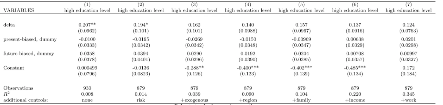
Table 1: Descriptive statistics: patience and present bias

Parameter Average (St. Error) Min Max Percentile

5th 10th 25th 50th 75th 90th 95th

δ12−13(N= 955) 0.808 (0.160) 0.465 1 0.465 0.541 0.714 0.833 0.952 1 1

β(N= 930) 0.992 (0.185) 0.465 2.15 0.663 0.788 0.943 1 1.023 1.162 1.305

The individual discount rate on the later time horizon (choices between amounts in a year and in a year and a month, that we call patience) has a median / mean value of 20% / 30.1%, with a wide range between 0% and 115% (standard deviation: 32.9%).¹³ The corresponding numbers of the median and the mean for the earlier time horizon (choices between amounts now and in a month) are 22.5% and 34.3%. Using the classification of Meier and Sprenger (2012), 35.6% of our sample is present-biased, 28.1% is future-biased, and the rest (36.3%) is time-consistent. The share of present-biased individuals is close to those found by Meier and Sprenger (2010) (36%), Ashraf et al. (2006) (about 27%) and Horn and Kiss (2018) (30%) for non-representative samples from the US, Phillipines and Hungary. Table 1 is similar in structure to table 3 in Bradford et al.

(2017) and the distributions are comparable.

Our risk measure is the percentage of the endowment that the respondent places as a bet. Our task is very similar to the one used in Gneezy and Potters (1997). Charness and Gneezy (2012) review numerous studies that use this task and find that participants tend to invest (bet in our case) about 50-70% of their endowment. We carried out the same task in a classroom experiment with university students and they risked on average 48.3% of their endowment (see Horn and Kiss, 2018). In our current survey individuals on average risked 38.5% of their endowment, which is somewhat lower than levels found in the literature. This may be due to the fact that in most of those experiments university students were the participants, who are not representative of the population.¹⁴Gong and Yang (2012) study villagers in China and they report similarly low (and even lower) levels using a similar risk elicitation method.

13 Frederick et al. (2002) report a similarly wide range of individual discount rates in their survey.

14 There are studies (e.g. Dohmen et al., 2010, 2018b) that document a positive relation between cognitive abilities and risk taking. Since arguably university students have higher cognitive abilities than the representative population, this may explain why we observe a lower level of risk taking. Note also that people under age 40 and with a tertiary degree risk 54,5% of their endowment in our sample, as well.

(15)

Using pairwise correlation, we find that patience (δ) and ourβ variable are negatively correlated (r=-0.38), that means that those who are less patient, are more likely to suffer from present bias in our sample. Note that this finding is somewhat artificial as a higherδ₁₂₋₁₃(our patience measure) implies that β is smaller conditional on δ₀₋₁. Note, however, asδ₁₂₋₁₃ and δ₀₋₁ are positively but not perfectly correlated (r=0.66), the varience ofβ is not zero. We also document a significant and positive correlation (r=0.11) between patience and risk tolerance, suggesting that more patient individuals in our sample tend to be less risk averse.¹⁵We detect some positive association between the present-bias variable (β <1) and risk tolerance, as present-biassed individuals risk 6% more of their endowments (p-value=0.004) compared to time-consistent people, but also future-biased individuals (when β >1) risk 6% more than their time-consistent peers (p=0.008).

To validate our measures, we briefly consider if we are able to find correlations reported in the literature in our data. A robust finding in the literature is that women are more risk averse (see for instance Croson and Gneezy (2009) or Bertrand (2011)).¹⁶ We find that women tend to be aproximately 10% more risk averse, which is a sizable and significant difference, that holds even if we control for the available individual characteristics. Dohmen et al. (2011) uses a large, representative German survey and find that older individuals tend to be less risk taking, a finding that we share.¹⁷ Noussair et al. (2013) using Dutch data report that more religious people are more risk averse. We find the same relationship in our data. Overall, we believe that our preference measures are meaningful.

4 Results

We present our results using coefficient plots as these show in a clear way if a variable associates with the outcome of interest or not. The coefficient plots visualize the estimation of the coefficient with the corresponding standard errors. We relegate the corresponding OLS regression outputs to section C in the Appendix.

In case of each domain, we estimate various models. In the first model we only add time preferences (that is,δand the two dummies related to time inconsistency - present bias (β <1) and future bias (β >1)).¹⁸

Then, in later models we add more and more controls. The first control is risk tolerance, measured by our preference task (ses section 2.1). Then we include a set of variables that we call exogeneous controls. These include age, age squared, if the respondent is female, and if the interviewer believes that the respondent is of Roma origin. The next set of control variables that we call region include dummies for the NUTS2 regions of Hungary and the type of settlement the respondent lives in.¹⁹ The fourth set of control variables are related tofamily and contains dummies related to the marital status (single, married, separated, living with partner, widow, divorced) and the number of children of the respondent. We have also control variables associated

15 As mentioned earlier, Leigh (1986) and Anderhub et al. (2001) reported the same finding, but there are papers that fail to find such correlation.

16 There are exceptions as for instance Harrison et al. (2007) do not find gender differences in risk aversion in a representative Danish sample.

17 Findings are varied as Tanaka et al. (2010) reports similar results as we do, however Harrison et al. (2007) document opposite findings.

18 Note that if we employed only the present bias dummy and did not control for future bias, then we would compare present bias to time consistencyand future bias. We believe that controlling for future bias allows us to gain a more accurate picture about the effect of present bias.

19 Regarding the regions, we have six dummies for the NUTS3 regions of Hungary, the baseline region being Central Hungary. We control for settlement type using three dummy variables (town, city, Budapest), the baseline being village.

(16)

witheducation including dummies if the respondent has a higher than basic education and if the respondent has a tertiary education degree. The set of control variables related toincomecontain information on the income level, on the wealth level (as detailed earlier in section 2.2.3) and on financial difficulties (having experienced problems paying utility bills or repaying mortgages or other outstanding loans, see section 2.2.4). The last set of control variables is related towork and has information on if the respondent works in the private / public sector and her employment status (e.g. unemployed, employee, employed, inactive etc.).

The sequence in which we presented our sets of control variables in the previous paragraph reflects the order as we include them into the regressions. Note that each new regression adds a new set of control variables to the ones that appeared in the previous regressions. Notice also that we will leave out the control variables that are directly related to the dependent variable. Thus, for instance, we do not control for education when we study which variables affect educational attainment. The coefficient plots visualize the effects at the 10 / 5% significance levels using thick / thin lines. Section C in the Appendix contains the coefficients and their significance of the variables of interest. We provide also an online appendix (section E) that contains the regressions with all the variables.

For the sake of completeness, in the figures we also show the effect of future bias. Not much is known about future bias, neither theoretically, nor empirically.²⁰ Since there is no relevant existing literature on future bias, we did not formulate any hypotheses and we will only comment on its effect when it is noteworthy in our view.

4.1 Educational attainment

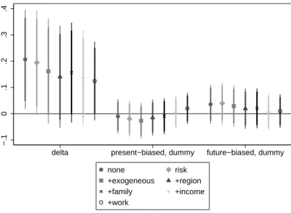
Figure 1 shows the effect of time preferences on the probability of obtaining a degree. Patience (delta) has the expected effect on educational outcome: the more patient a respondent, the more likely that she has a diploma. Moreover, the effect is marginally significant also when we control for risk attitudes. However, as we add more control variables, the effect ceases to be significant. Interestingly, it becomes marginally significant again when adding all the control variables. Present bias does not have a significant effect in any of the specifications and does not even show a consistent pattern.

We carry out the same analysis at the other end of the education attainment distribution.

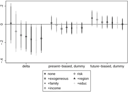
That is, we investigate if time preferences are different for people with at most an elementary school degree. Interestingly, Figure 2 is not the mirror image of Figure 1, because we see that patience is not only significant when considering alone or with risk attitudes, but also as we add other control variables. The level of significance decreases gradually, but even after including all the control variables, patience is marginally significant at the 10% level. That is, even after taking into account a wide range of variables the more patient an individual, the less probable it is that she drops out from education early. The asymmetric effect of patience on educational outcomes suggests that it has a larger role in escaping low educational attainment than to achieve a university degree.

The sign of the present bias dummy is also consistently above zero and in some cases it is even significant. It loses significance when we control for income and work that are ’bad controls’

in the sense that they are highly correlated with educational attainment. This suggests that present-biased individuals are more likely to end up without a high school degree, in line with our hypothesis.

Finding 1 (education): Patience seems to be important in escaping low educational attainment even after controlling for a host of variables, but less important when considering attaining

20 A notable exception is Takeuchi (2011).

(17)

Fig. 1: The association of time preference and the probability of obtaining a tertiary degree

−.10.1.2.3.4

delta present−biased, dummy future−biased, dummy

none risk

+exogeneous +region

+family +income

+work

Note: Coefficient plots of the variables of interest. Coefficients with 10 / 5% significance levels, from Table 2 in Appendix C

Fig. 2: The effect of time preference on the probability of failing to obtain a high-school degree

−.6−.4−.20.2

none risk

+exogeneous +region

+family +income

+work

(18)

a diploma. Present bias seems to have a consistent positive association with failing to obtain a higher than elementary degree, but has a rather erratic effect when investigating its role in obtaining a diploma.

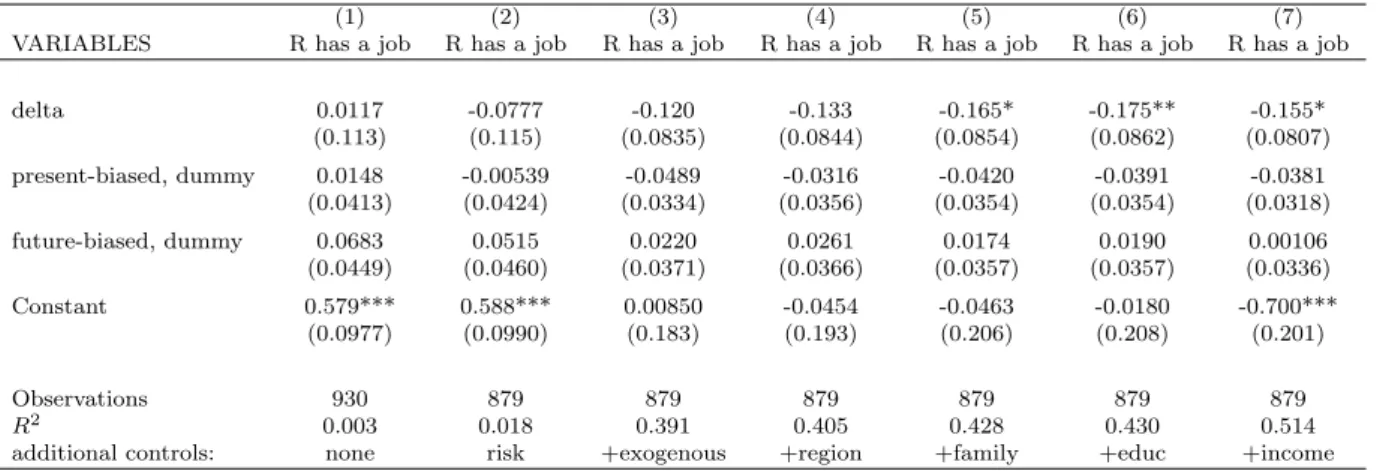
4.2 Unemployment

We hypothesize a positive (negative) relationship between patience (present bias) and being employed. We exclude from this analysis those individuals who are retired, on maternal leave or are students, because they are not active on the labour market.

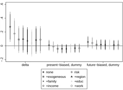
Fig. 3: The association of time preference with the probability of employment

−.4−.20.2

none risk

+exogeneous +region

+family +educ

+income

Figure 3 shows that being employed is generally negatively correlated with patience and the effect is often significant after we take into account the risk, exogenous, region and family controls. Present bias has an insignificant association with being employed. Surprisingly, we not only do not find any support for our hypotheses related to employment and patience, but we find the opposite.

We attempted various different specifications informed by the following arguments. One may argue that some individuals may prefer to be unemployed rather than having a job that they dislike, so they possibly would wait to have an appealing offer. This may make unemployment spells longer and actually may make the effect of patience weaker. Since potentially wealthy or well-off individuals could afford to wait, we excluded them from the analysis and rerun the regressions for the respondents below the mean / median income. Though the numbers change somewhat, we see basically the same qualitative pattern. As a further check, we excluded the self-employed individuals from the analysis, but the results do not change here either.

(19)

4.3 Income and wealth

Based on the literature, we hypothesize a positive correlation between patience and income (and wealth), and we expect a negative relationship between present bias and income (and wealth).

Fig. 4: The association of time preference with income

−40000−200000200004000060000

none risk

+exogeneous +region

+family +educ

+work

We do not observe strong associations between time preferences and income. There is a marginal positive effect of patience (as expected) when omitting other variables, but the effect disappears as control variables are included in the regressions. Similarly, the effect of present bias is not significantly different from zero in any specification.

The effect of patience on wealth is in line with our expectations. We see a significant positive effect when considered alone or even when we control for risk attitude. The effect remains strong after controlling for age, gender and ethnicity and becomes marginally significant if we add regional and settlement type dummies. If we add more control variables oneducation andwork, the effect ceases to be significant. However, these latter two, again, are probably bad controls as they directly impact wealth. Having this in mind, we would argue that patience could be a strong predictor of wealth. Present bias always has a negative sign as expected, and is also significant if we take risk, exogenous, region and family into account. This, however, also indicates that present-biassed individuals tend to accumulate less wealth over their life.

Finding 3 (income and wealth): Patience has mostly a positive, but generally insignificant association with income. For wealth the positive association is much more straithforward and significant in many specifications. The effect of present bias is almost always negative on both income and wealth (as expected), but this effect is significant only marginally in some specifications, and mainly for wealth.

(20)

Fig. 5: The association of time preference with wealth

−.50.51

none risk

+exogeneous +region

+family +educ

+work

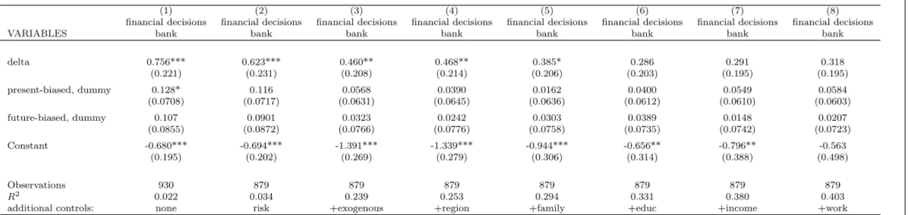
4.4 Financial decisions and financial difficulties 4.4.1 Banking and saving decisions

Based on the literature, we expect that more patient individuals tend to i) use more the basic banking services, ii) save more. Regarding present bias, we expect to see the opposite associations.

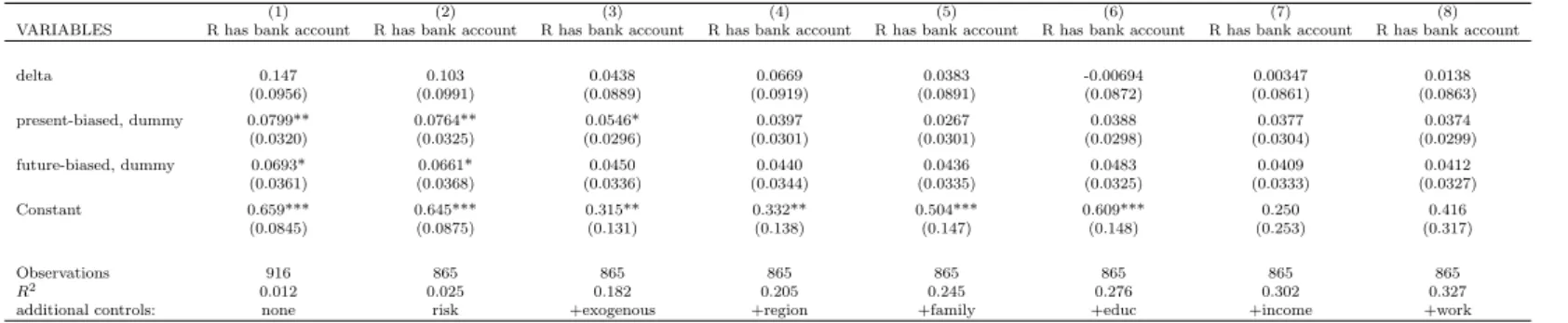
In line with our hypotheses, we observe a steady positive association of patience with banking decisions in Figure 6. The significance subsides somewhat as we add more and more controls, but the effect remains at least marginally significant even after including all controls. The present bias dummy has a significant and positive effect on banking decisions in the first regressions. This positive effect is not in line with our expectations.²¹When looking at the individual components of the index, in the case of having a bank account, patience does not play a significant role, present bias shows a significant and positive effect (in contrast to our conjecture) in the first regressions, but not after controlling for region. Concerning banking card, patience exhibits a consistent positive effect that is significant without controls, but the significance disappears after controlling forexogenous factors. Present bias also has an unexpected consistent positive effect that is marginally significant without controls and when only risk tolerance is included as control.

For details, see Tables 12 and 13 in section D of the Appendix.

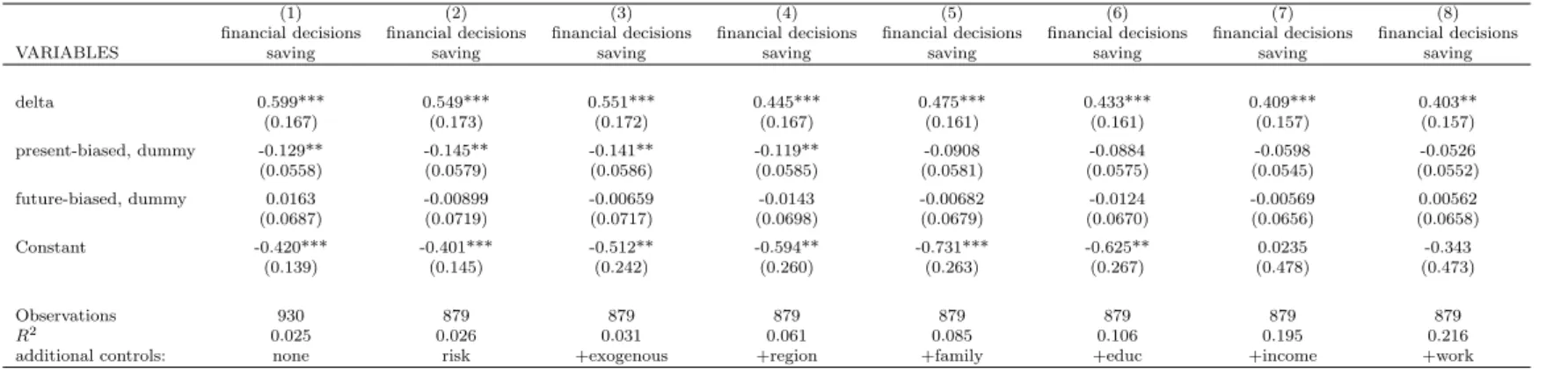
When investigating saving decisions, in line with our hypotheses patience has a significant positive effect, even if we include as controls all the variables that we have information about.

Present bias also has the expected negative effect and it is significant even if we control for risk

21 A potential explanation is that if an individual is aware of suffering from present bias, then she may use commitment devices to deal with this problem (e.g. Ashraf et al., 2006). Our data does not allow to check if this is the case here.

(21)

Fig. 6: The association of time preference with banking decisions

0.511.5

none risk

+exogeneous +region

+family +educ

+income +work

Fig. 7: The association of time preference with saving decisions

−.50.51

none risk

+exogeneous +region

+family +educ

+income +work

(22)

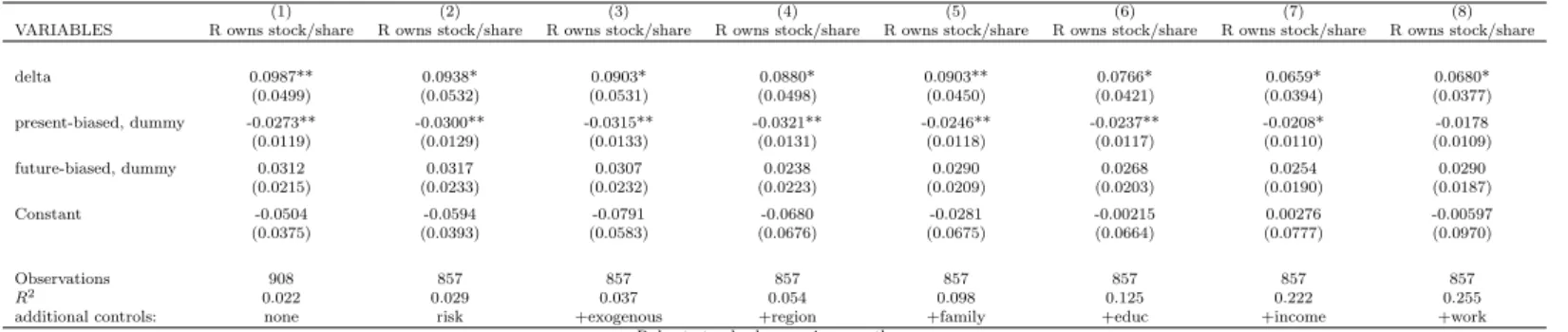
attitude, exogenous variables and region. When considering separately the components of the saving index, then we find that patience has a consistent and positive effect on the ownership of stocks that is significant at least at 10% throughout the regressions. Hence, more patient individuals are more likely to own stocks. The effect of present bias is also in line with the expectations, that is, present-biased individuals are less likely to own stocks. This effect is significant in all, but the last specifications. When turning to retirement savings, a similar but stronger pattern emerges. Patience shows a very strong positive effect throughout the regressions. Even if we control for all the variables, its effect is still significant at the 1%. Present bias has the expected negative effect and it is at least marginally significant in almost all specifications. Considering having a life insurance, patience has a consistent positive effect (as expected) that proves to be significant in all regressions. However, present bias does not seem to play a role as it is not significant in any specification. For details, see Tables 14, 15 and 16 in section D of the Appendix.

Finding 4 (financial decisions): Regarding banking decisions, patience has a consistent positive and significant association with the outcome, while present bias does not seem to play a role. When considering separately the components of banking decisions, having a bank account is not affected by patience and is positively influenced by present bias, the influence being significant only when at mostexogeneousvariables are considered. Concerning having a bank card, patience has a consistent positive association that is significant when some control variables are added. Present bias is negatively associated with having a bank card, and the effect is significant only without controls and when we add risk attitudes, with more controls it ceases to be significant. Patience exerts a very strong positive and significant association with having savings.

The association is strongest for retirement savings, followed by life insurance and owning stocks.

We also observe that present-biased individuals are less likely to have savings, in general. This pattern is observed for stock ownership and retirement savings, but is absent in the case of life insurance.

4.4.2 Financial troubles

According to Figure 8 patience is not associated with financial troubles in our sample. The sign of the coefficient is consistently negative, suggesting that more patient individuals are less likely to suffer financial distress, but it has no significant effect in any of the specifications. However, present-biased individuals tend to have more financial troubles. The coefficient of the present bias dummy is statistically significant in all specifications. The results show that being present-biased relative to time-consistent increases the likelihood of suffering financial troubles by 16-18%. This result is very similar to that found by Meier and Sprenger (2010) who study credit card borrowing and find that individual discount factors do not explain credit card debt, while present bias does.

Finding 5 (financial troubles): Patience associates in a consistently negative manner with the occurrence of financial troubles (as expected), however the association fails to be significant. Present bias has the expected positive effect on financial troubles, moreover this effect is significant even if we add all the control variables.

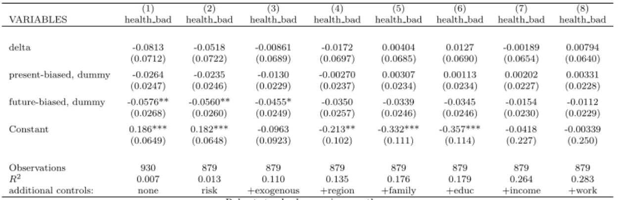
4.5 Health

Following Bradford et al. (2017), we form two dummy variables based on the answers given to the self-reported health question in the survey. If the respondent chooses one of the two categories that report an inferior health, then we say that the individual has bad health. Similarly, we construct a dummy variable standing for good health. Based on the literature, we expect a positive (negative) relationship between patience (present bias) and self-reported good health.

(23)

Fig. 8: The association of time preferences with financial troubles

−.6−.4−.20.2.4

none risk

+exogeneous +region

+family +educ

+income +work

In Figure 9 we do not see any association of patience or present bias with bad health. Pa- tience seems to have a generally negative association (as expected), but fails to be significant.

The association of present bias is consistently negative (contrary to our expectations) and not significant in any of the specifications.²²

Figure 10 indicates that without control variables, patience associates significantly and positively with good health, as expected. The significance goes away as we add control variables, but reassuringly we see that the coefficient has a consistent positive sign. Present bias does not have a significant effect.

Finding 6 (health): We find weak evidence that more patient individuals are more likely to enjoy good health, but we fail to document any significant effect of patience on bad health or any influence of present bias on self-reported health.

5 Discussion

In this study we investigated the association between two aspects of time preferences (patience and present bias) and life outcomes in five domains. Patience has the expected effect in most of the cases in terms of exhibiting consistently the expected sign and being significant in at least some specifications. The associations are the strongest with escaping low educational attainment, wealth, banking and saving decisions and financial troubles. Only in the case of unemployment we observe unexpected signs.

22 Interestingly, being future-biased is significantly correlated with bad health in some specifications especially without controls: future-biased individuals are less likely to suffer bad health.

(24)

Fig. 9: The association of time preference with having bad health

−.2−.10.1.2

none risk

+exogeneous +region

+family +educ

+income +work

Fig. 10: The effect of time preference on having good health

−.20.2.4.6

none risk

+exogeneous +region

+family +educ

+income +work

(25)

Present bias seems to be less important, as it has low to no association with many outcomes.

It has the expected sign and is signifcant in at least some specifications only when considering escaping the low educational outcome, banking and saving decisions, and financial troubles.

There are at least two potential explanations why the effect of present bias is less pronounced than that of patience. First, if an individual is aware that she suffers from present bias, then she may use commitment devices (e.g. Bryan et al., 2010) to overcome her problem as we already pointed out in the case of banking decisions. We cannot observe the use of commitment devices, so in principle we cannot discard their effect. However, we could not come up with a good story why commitment devices help in the areas where we do not see an effect of present bias, but not in the other domains. Further studies should investigate, for instance, if commitment devices in financial services and issues could dampen the negative effect of present bias. Second, Augenblick et al. (2015) - among others - argue that present bias may be more marked in case of consumption goods than for monetary flows. We do not consider real consumption goods and actually we observe that present bias has some effect in issues involving money (banking, saving and financial difficulties), so this explanation seems to have no importance in our case.

We consider a strength of our study that it uses a representative sample that allows us to draw firmer conclusions about the effect of time preferences on life outcomes. More such representative samples with more respondents under different elicitation methods and incentive schemes would be welcome so that we obtain a more robust knowledge on how patience and time inconsistency associate with relevant outcomes in life. Given a more conclusive knowledge we will able to come up with adequate policy interventions. Some steps have been made in that direction already. In line with the early childhood intervention literature (see for instance Zigler, 2000; Elango et al., 2015), Alan and Ertac (2018) design an intervention to foster patience. The intervention indeed leads to more patient intertemporal choices in case of the treated students and has a persistent positive effect on school performance. Our study (and others in this literature) suggest that such interventions may have effect in other domains as well.

References

Abdellaoui M, Gutierrez C, Kemel E (2018) Temporal discounting of gains and losses of time:

An experimental investigation. Journal of Risk and Uncertainty 57(1):1–28

Alan S, Ertac S (2018) Fostering patience in the classroom: Results from randomized educational intervention. Journal of Political Economy 126(5):1865–1911

Anderhub V, G¨uth W, Gneezy U, Sonsino D (2001) On the interaction of risk and time preferences: An experimental study. German Economic Review 2(3):239–253

Andersen S, Harrison GW, Lau MI, Rutstr¨om EE (2008) Eliciting risk and time preferences.

Econometrica 76(3):583–618

Andersen S, Harrison GW, Lau MI, Rutstr¨om EE (2014) Discounting behavior: A reconsidera- tion. European Economic Review 71:15–33

Andreoni J, Sprenger C (2012) Risk preferences are not time preferences. American Economic Review 102(7):3357–76

Andreoni J, Kuhn MA, Sprenger C (2015) Measuring time preferences: A comparison of experimental methods. Journal of Economic Behavior & Organization 116:451–464

Angeletos GM, Laibson D, Repetto A, Tobacman J, Weinberg S (2001) The hyperbolic consumption model: Calibration, simulation, and empirical evaluation. Journal of Economic Perspec- tives 15(3):47–68

Ariely D, Wertenbroch K (2002) Procrastination, deadlines, and performance: Self-control by precommitment. Psychological Science 13(3):219–224