Photodynamical analysis of the triply eclipsing hierarchical triple system EPIC 249432662

(1)

Advance Access publication 2018 November 22

Photodynamical analysis of the triply eclipsing hierarchical triple system EPIC 249432662

T. Borkovits ,

^1,2^‹

S. Rappaport,

³

T. Kaye,

⁴

H. Isaacson,

⁵

A. Vanderburg,

^6,7

† A. W. Howard,

⁸

M. H. Kristiansen,

^9,10

M. R. Omohundro, ‡ H. M. Schwengeler, ‡ I. A. Terentev, ‡ A. Shporer,

¹¹

H. Relles,

¹¹

S. Villanueva Jr,

^11,12

T. G. Tan,

¹³

K. D. Col´on,

¹⁴

J. Blex,

¹⁵

M. Haas,

¹⁵

W. Cochran

⁷

and M. Endl

⁷

1Baja Astronomical Observatory of Szeged University, H-6500 Baja, Szegedi ´ut, Kt. 766, Hungary

2Konkoly Observatory, Research Centre for Astronomy and Earth Sciences, Hungarian Academy of Sciences, Konkoly Thege Mikl ´os ´ut 15-17, H-1121 Budapest, Hungary

3Department of Physics, Kavli Institute for Astrophysics and Space Research, M.I.T., Cambridge, MA 02139, USA

4Raemor Vista Observatory, 7023 E. Alhambra Dr., Sierra Vista, AZ 85650, USA

5Department of Astronomy, University of California at Berkeley, Berkeley, CA 94720-3411, USA

6Harvard-Smithsonian Center for Astrophysics, 60 Garden Street, Cambridge, MA 02138 USA

7Department of Astronomy, The University of Texas at Austin, 2515 Speedway, Stop C1400, Austin, TX 78712

8Astronomy Department, California Institute of Technology, MC 249-17, 1200 E. California Blvd, Pasadena, CA 91125, USA

9DTU Space, National Space Institute, Technical University of Denmark, Elektrovej 327, DK-2800 Lyngby, Denmark

10Brorfelde Observatory, Observator Gyldenkernes Vej 7, DK-4340 Tølløse, Denmark

11Kavli Institute for Astrophysics and Space Research, M.I.T., Cambridge, MA 02139, USA

12Department of Astronomy, The Ohio State University, Columbus, OH 43210, USA

13Perth Exoplanet Survey Telescope, Perth, Western Australia 6010, Australia

14NASA Goddard Space Flight Center, Exoplanets and Stellar Astrophyscs Laboratory (Code 667), Greenbelt, MD 20771, USA

15Astronomisches Institut, Ruhr Universit¨at, 44780 Bochum, Germany

Accepted 2018 November 20. Received 2018 November 20; in original form 2018 September 3

A B S T R A C T

Using Campaign 15 data from theK2 mission, we have discovered a triply eclipsing triple star system: EPIC 249432662. The inner eclipsing binary system has a period of 8.23 d, with shallow∼3 per cent eclipses. During the entire 80-d campaign, there is also a single eclipse event of a third body in the system that reaches a depth of nearly 50 per cent and has a total duration of 1.7 d, longer than for any previously known third-body eclipse involving unevolved stars. The binary eclipses exhibit clear eclipse timing variations. A combination of photodynamical modeling of the light curve, as well as seven follow-up radial velocity measurements, has led to a prediction of the subsequent eclipses of the third star with a period of 188 d. A campaign of follow-up ground-based photometry was able to capture the subsequent pair of third-body events as well as two further 8-d eclipses. A combined photo- spectro-dynamical analysis then leads to the determination of many of the system parameters.

The 8-d binary consists of a pair of M stars, while most of the system light is from a K star around which the pair of M stars orbits.

Key words: binaries: close – binaries: eclipsing – stars: individual: EPIC 249432662.

1 I N T R O D U C T I O N

Hierarchical triple stellar systems and/or subsystems form a small but very important subgroup of the zoo of multiple stellar systems.

E-mail:borko@electra.bajaobs.hu

†NASA Sagan Fellow.

‡Citizen Scientist.

Their significance in the formation of the closest main-sequence binary systems (see e.g. Eggleton & Kiseleva-Eggleton2001; Fab- rycky & Tremaine2007; Naoz & Fabrycky2014; Maxwell & Krat- ter2018, and further references therein) is widely acknowledged.

Hierarchical triples have also been hypothetized to play a significant role in the formation of some kinds of peculiar objects, such as blue stragglers (Perets & Fabrycky2009), low-mass X-ray binaries (Shappee & Thompson2013), and some peculiar binary pulsars

2018 The Author(s)

Downloaded from https://academic.oup.com/mnras/article-abstract/483/2/1934/5199225 by guest on 20 December 2018

(2)

Figure 1. Pole-on view of the hierarchical triple star system EPIC 249432662. The red and blue curves represent the motions of the Ba and Bb stars of the ‘inner’ 8-d binary orbit in their 188-d ‘outer’ orbit about the center of mass (CM) of the triple system (located atX=Y=0).

The thin grey curve marks the locus of CM points for the 8-d binary. The green curve is the 188-d ‘outer’ orbit of star A, the third star that comprises the system. The thin green lines denote the major and minor axes of the orbit of star A, while the thin green arrow indicates the direction of motion along the orbits. Thicker sections of the orbits represent the arcs on which the three stars were moving during the ‘great eclipse’, observed with theKepler spacecraft around BJD 2 458 018. The black arrow that connects these arcs is directed toward the observer.

(see e.g. Portegies Zwart et al.2011). They might even have a role in driving two white dwarfs to merger in that scenario for type Ia supernova explosions (Maoz, Mannucci & Nelemans2014).

In the case ofhierarchicaltriples, one of the three mutual distances among the three components of the system remains substan- tially smaller than the other two distances for the entire lifetime of the triple. Therefore, the dynamics of the triple can be well ap- proximated with the (slightly perturbed) Keplerian motions of two

‘binaries’: an inner or close binary, formed by the two components having the smallest separation, and an outer or wide ‘binary’, consisting of the centre of mass of the inner pair and the more distant third object (see Fig.1for a schematic diagram).¹For most of the known hierarchical triple star systems, with large period ratios for the ‘outer binary’ to ‘inner binary’, departures from pure Keplerian motion are expected to become significant only on time-scales of decades, centuries, or even millenia, i.e. over much longer intervals than the length of the available observational data trains. However,

1In this paper, we use the following notations. The orbital elements of the inner and outer orbits are subscripted by numbers ‘1’ and ‘2’, respectively.

Regarding the three stars, we label them asA,Ba, andBb, whereAdenotes the brightest and most massive component, i.e. the distant, third star, while BaandBbrefer to the primary and the secondary components of the close, inner 8-d binary. When we refer to physical quantities of individual stars, we use these subscripts. In such a way, for example,mAormBastands for the masses of componentsAorBa, respectively, butmBdenotes the total mass of the inner binary, (mBa+mBb), whilemABrefers to the total mass of the entire triple system.

there is an important subgroup of the hierarchical triple systems, the so-called ‘compact hierarchical triples’ (CHT), which have smaller ratios of ‘outer’ to ‘inner’ periods and, occasionally, also smaller characteristic orbital dimensions. These may show much shorter time-scale and well-observable dynamical (or other kinds of) interactions so that they allow us to promptly determine many of the important dynamical and astrophysical parameters of these systems.

For example, a careful analysis based (partly) on the dynamically perturbed pulsar timing data of the millisecond pulsar PSR J0337+1715 orbiting in a peculiar CHT consisting of two white dwarfs in addition to the pulsar component has led to the accurate determination of the masses of all three objects, as well as the spatial configuration of the triple (Ransom, Stairs & Archibald 2014). Similarly, as shown by Borkovits et al. (2011,2015), if the close pair of a CHT happens to be an eclipsing binary (EB), the dynamical perturbations of the third companion on the orbital motion of the EB manifest themselves in intensive and quasi-cyclic eclipse timing variations (ETVs) on the time-scale of the orbital period of the outer component. The analysis of this effect makes it possible to determine not only the complete spatial configuration of the triple system but also the masses of the three objects.

As an application of the latter ETV analysis method, Borkovits et al. (2016) investigated 62 such CHTs in the original field of the Keplerspace telescope (Borucki, Koch & Basri2010) where the inner binary was an EB, and the dynamical interactions were significant. They were able to determine many of the system parameters, including the mutual inclination of the planes of the inner and outer orbits, which is a key parameter from the point of view of the different triple star formation theories (see e.g. Tokovinin 2017). In the same paper the authors identified an additional 160 CHTs through the traditional light-travel time effect (LTTE; see e.g. Irwin1959) and, in total, they found∼104 CHTs with outer orbital periodP2 1000 d; this provides by far the most popu- lated sample of hierarchical triple stars at the lower end of their outer period distribution. They pointed out a significant dearth of ternaries withP2200 d, and concluded that this fact cannot be explained with observational selection effects. This latter result is in accord with the previous findings of Tokovinin et al. (2006) on the unexpected rarity of (the mostly spectroscopically discovered) triple systems in the period regimeP2<1000 d, whose shortage is more explicit amongst those CHTs which contain exclusively solar mass and/or less massive components (Tokovinin2014). Therefore, investigations of such systems are especially important.

A very narrow subgroup of CHTs that offers further extraor- dinary possibilities for accurate system parameter determinations are those triples, which exhibit outer eclipses. These systems have a fortuitous orientation of the triple system relative to the observer whereby, occasionally, the distant third component eclipses one or both stars of the inner close binary or, vice versa, it is eclipsed by them. Such phenomena had never been seen before the advent of the Kepler era. The Kepler space telescope’s 4- yr-long, quasi-continuous observations, made with unprecedented photometric precision have, however, led to the discovery of at least 11 CHTs exhibiting outer eclipses, and a similar number of circumbinary transiting extrasolar planets. The latter group, though dynamically similar, are not considered in the following list of CHTs. These are KIC 05897826 (=KOI-126; Carter, Fab- rycky & Ragozzine2011), KIC 05952403 (=HD 181068; Derekas, Kiss & Borkovits 2011), KICs 06543674, 07289157 (Slawson, Prˇsa & Welsh 2011), KIC 02856960 (Armstrong et al. 2012;

Marsh, Armstrong & Carter2014), KIC 02835289 (Conroy et al.

2014), KICs 05255552, 06964043, 07668648 (Borkovits et al.

(3)

2015), KIC 09007918 (Borkovits et al.2016), and KIC 0415061 (=HD 181469), the latter of which is possibly at least a quintuple system (Shibahashi & Kurtz2012; Hełminiak et al.2017). For 10 of these 11 CHTs, besides the outer eclipses, the inner binary also shows regular eclipses; hence, we call these CHTs ‘triply eclipsing systems’. (The only exception is KIC 02835289, where the inner binary is an ellipsodial light variable.) Though the much shorter duration of theK2observations is less favourable in regard to the discovery of systems with outer eclipses, another triply eclipsing CHT, HD 144548 was also identified in the C2 field of the extended K2mission (Alonso et al. 2015). Furthermore, recently, Hajdu, Borkovits & Forg´acs-Dajka (2017) reported the discovery of two additional triply eclipsing CHTs, namely CoRoTs 104079133 and 221664856 amongst the EBs observed by the CoRoT space telescope (Auvergne et al.2009).

Precise modeling of the brightness variations of these CHTs, especially during each outer eclipse, is a great challenge but, on the other hand, it offers huge benefits. This is so because the light curve is extremely sensitive to the complete configuration of the triple. As a consequence, even in the case where the outer orbit is wide enough to safely allow for the elimination of any dynamical perturbations in the analysis of accurate ETV and/or radial velocity (RV) curves, the same cannot be done for the light-curve solution. This is true because dynamically induced departures in the positions and velocities of the three bodies relative to a purely Keplerian motion, even if they are very small, will strongly affect all the characteristics of the forthcoming outer eclipses. Therefore, the accurate modeling of such systems, in most cases, requires a photodynamical approach, including the complete numerical integration of the motion of the three bodies, together with the simultaneous analysis of the light curve(s) (and, if it is available, the RV curve[s], as well), as was carried out by, e.g. Carter et al. (2011), for KOI-126 and Orosz (2015), for KIC 07668648.²

In this paper we report the discovery and present the photodynamical analysis of the new triply eclipsing CHT EPIC 249432662 (= 2MASS J15334364-2236479, UCAC4 337-074729). The system was observed during Campaign 15 of theK2mission. Besides the regular,∼3 per cent deep eclipses belonging to an 8.23-d period, slightly eccentric EB, theKeplerspacecraft has observed an additional, 1.7-d-long, irregularly shaped fading event with an amplitude of almost 50 per cent which we assumed to be an outer eclipse due to the presence of a third, distant, gravitationally bound stellar component. Ground-based spectroscopic and photometric follow-up observations have confirmed our assumption and made it possible to carry out a complete, joint photo-spectro-dynamical analysis of this 188.3-d-outer-period, triply eclipsing CHT, including the simultaneous joint analysis ofK2and ground-based light curves, the ETV curve (derived from the photometric observations), and the ground-based RV curve, all accompanied by the numerical integration of the motion of the three bodies. We derive many of the parameters for this system. The paper is organized as follows. In Section 2 we describe the 80-dK2observation of EPIC 249432662.

Existing archival data on the target star are summarized in Section 3.

Our two ground-based photometric follow-up campaigns, which led to the successful detection of further outer eclipses, are discussed

2In addition to KIC 07668648, J. Orosz has also successfully applied the same combined photodynamical approach to other CHTs amongst the Kepler-discovered EBs (e. g. to KIC 10319590) that did not exhibit outer eclipses, but the rapid eclipse depth variations and the features of the ETV and RV curves have allowed him to infer accurate system parameters.

in Section 4, while the ETV data determined from both the K2 and ground-based photometry are briefly described in Section 5.

In Section 6 we present our spectroscopic RV follow-up observations. We then use our improved photodynamical software package to model and evaluate the satellite and ground-based light curves, ETV curves, and RV results simultaneously (see Section 7). In Sec- tion 8 we discuss some of the astrophysical and orbital/dynamical implications of our solutions. We summarize our findings and draw some conclusions in Section 9. Finally, we discuss some practical details of our photodynamical code in Appendices A and B.

2 K2 O B S E RVAT I O N S

Campaign 15 (C15) of theK2mission (Howell et al.2014) was directed toward the constellation Scorpius between 2017 August 23 and 2017 November 20 for approximately 87 uninterrupted days. At the end of November, theK2Guest Observer (GO) Office made the C15 raw cadence pixel files (RCPF) publicly available on the Barbara A. Mikulski Archive for Space Telescopes (MAST).³ We utilized the RCPF in conjunction with theKADENZAsoftware package⁴(Barentsen & Cardoso2018), in a manner similar to re- centK2-discoveries (see e.g. Christiansen et al.2108; David et al.

2018; Yu et al.2018), combined with custom software in order to generate minimally corrected light curves. Due to limited processing power, some of us (MO, IT, HMS, MHK) generated a series of short-baseline C15 preview light curves, and carried out manual surveys with thelctoolssoftware (Kipping et al.2015). The first C15 preview search identified EPIC 249432662 (proposed by GO15083, Coughlin)⁵as a likely 8-d eclipsing binary, while our second extended preview light curve identified an additional single, deep, compound eclipsing event of long duration centered at BJD

=2458 018.

Once the calibrated Ames data set was released, we downloaded all availableK2extracted light curves common to Campaign 15 from the MAST. We utilized the pipelined data set of Vanderburg &

Johnson (2014) to construct the light curve, which is presented in Fig.2; the top panel shows the data for all 80 d of theK2observation, whereas the bottom panel shows a 10-d zoom-in around the large eclipse that we dub the ‘great eclipse’ (or ‘GE’). The two nearly equal-depth eclipses from the 8-d binary are also clearly evident.

When looked at in the expanded view, the ‘great eclipse’ is seen to be composed of a deep and slightly asymmetric portion (here called

‘GE1’) and a sharp (i.e. short-duration) extra dip (called ‘GE2’) near the minimum of the event.

Note, however, that in our photodynamical analysis (see Sec- tion 7), we used a ‘flattened’ version of the light curve that differs from the one shown in Fig.2by having the long-term trend and low-frequency variability removed. The procedure is to iteratively fit a basis spline (B-spline) with breakpoints every 1.5 d to the light curve with the 3σ outliers (including, of course, the eclipses) removed from the fit. This process is repeated until convergence is achieved (see Vanderburg & Johnson2014). The eclipses, including the great eclipse, are then added back to the spline fit.

We have examined both theK2pixel-level data and the PANStarrs image (Chambers et al.2016) of the field to check on ‘third-light’

contamination to theK2light curve from neighbour stars. We utilized the pixel reference function ofKepler(on the module with the

3http://archive.stsci.edu/k2/data search/search.php

4https://github.com/KeplerGO/kadenza

5https://keplerscience.arc.nasa.gov/data/k2-programs/GO15083.txt

(4)

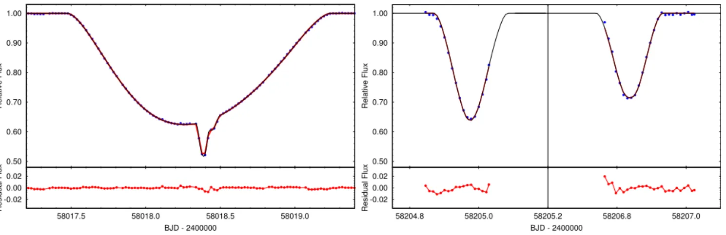
Figure 2. K2light curve of EPIC 249432662 from Campaign 15.Top panel:

full 80-d light curve;bottom panel:10-d zoom-in around the long, deep, and structured eclipse of the third star by the inner binary.

Great Eclipser; Bryson et al.2010), which gives the contribution from a given star as a function of distance from the maximum in flux. The nearest star that could add contaminating light is 15away and is only∼20 per cent the brightness of the target. The contribution from this star, according to the pixel reference function, is then no more than 0.1 per cent of the target star, and hence negligible.

Before doing any quantitative analysis, we qualitatively con- vinced ourselves that GE1 must be due to an eclipse of a third star in the system by one of the binary stars. This star would just happen to be moving in the same direction on the sky as the third star, and nearly at the same speed, so as to dramatically slow their relative motion and produce an eclipse that lasts for 1.7 d. By contrast, GE2 must be caused by the other star in the binary that is moving in theoppositedirection on the sky as the third star. We also concluded early on that the two stars in the binary must be of comparable mass, size, andTeff, based on the near equality of the two binary eclipses. Finally, we realized that there was just a limited set of stellar parameters that would allow for only one star in the binary to be able to block∼38 per cent of the system light.

In the remainder of the paper we focus on understanding this

‘great eclipse’ quantitatively and, in the process, extracting the system parameters.

3 A R C H I VA L DATA

The target star image, as a composite of all three stars, has aKe- plermagnitude of 14.93. The coordinates of the target star and its brightness in other magnitude bands from the blue to the WISE 3 band are summarized in Table1. The new Gaia DR2 release puts

Table 1. Photometric properties of EPIC 249432662.

Parameter EPIC 249432662

Aliases 2MASS J15334364-2236479

WISE J153343.62-223648.1 UCAC4 337-074729 Gaia DR2 6239702584685025280

RA (J2000) 15:33:43.639

Dec. (J2000) −22:36:48.07

Kp 14.93

B 16.57^a

V 15.46^a

G 14.92^b

r 14.95^a

i 14.45^a

J 12.83^c

H 12.25^c

K 12.09^c

W1 11.99^d

W2 11.96^d

W3 11.71^d

Distance (pc) 445±7^b

μα(mas yr⁻¹) −18.70±0.07^b

μδ(mas yr⁻¹) −10.82±0.05^b

Notes.^aUCAC4 (Zacharias et al.2013).^bGaia DR2 (Lindegren et al.2018).

c2MASS archive (Skrutskie et al.2006).^dWISE archive (Cutri et al.2013).

the target at a distance of 445±7 pc. This distance and the corresponding proper motions from Gaia DR2 are also listed in Table1.

Note, however, that despite the unprecedented astrometric precision of Gaia, the DR2 parallax, and therefore distance, for the present system should be considered as only a preliminary value, and should not be accepted without some caveats. The reason is that binary star solutions have not yet been incorporated into the DR2 results. In particular, since the orbital period of the outer orbit in our triple is P2∼188 d, which is almost exactly half of the orbital period of the Gaia satellite, the absence of corrections for the internal motions might be critical for our triple.

Based on the Gaia photometry and the source distance, the DR2 file on this object lists the star as having a radius of 0.86⁺₋^0.055_0.077R. Of course, this analysis is based on the assumption that there is one dominant star present, and the light from the two stars in the 8-d binary do not contribute much to the system light.

Under these assumptions we know at least that the third star is of K spectral type with a mass of∼0.7−0.8M, and lies quite close to the zero-age main sequence.

4 G R O U N D - B A S E D F O L L OW- U P O B S E RVAT I O N S

The history of our ground-based follow-up observations nicely il- lustrates the role of good fortune in a scientific endeavour. Our preliminary joint photodynamical runs, including theK2photome- try and the ETV curves derived from it, clearly demonstrated that the main features of theK2light curve can be well reproduced with a compact, dynamically active, triple stellar system in an almost coplanar configuration. However, due to the strong degeneracies among many of the orbital parameters in terms of the outer eclipsing pattern, we were unable to constrain the outer orbital period and, therefore, to predict the likely time(s) of the forthcoming outer eclipses. This situation changed dramatically after we obtained the fourth RV data point from 2018 March 22. This RV point made it possible to constrain the outer period with only an∼2–3-d un-

(5)

certainty and, therefore, to predict the most probable forthcoming outer eclipse times to within a range of only a few days. The most important consequence was that we then understood that the forthcoming outer eclipses should be occurring within 5–10 d of that time! Therefore, we had to urgently organize an international observing campaign with several observers from Arizona to Chile. We were thereby able to perfectly catch the next pair of ‘great (outer) eclipses’ almost exactly after the start of the follow-up ground-based observations.

JBO observations

The observations of the primary third-body eclipses were conducted with the Junk Bond Observatory by the author TGK. The telescope is an 80-cm Ritchie Chretien with an SBIG STL6303E CCD. 60-s unfiltered images were shot sequentially through the events. Darks, flats, and data images were reduced using theMAXIMDLsoftware by Bruce Gary.

The observations were carried out for 5 and 6 h on the evenings of 2018 March 27 and 29, respectively. By good fortune, both of the deep primary third-body eclipses were captured photometrically.

RoBoTT telescope observations

We have carried out photometry of the target star at the end of 2018 March with the ROBOTT telescope (formerly VYSOS6). The images are taken in two filters: sloanrandi, during the first night with exposure times of 30 s, and then later at 60 s. Typically nine images are combined with outlier rejection to remove cosmic rays.

The images are taken at the same sky position, and the source of interest is at the image center. While the FoV of the instrument is 2.7×2.7 deg, we extracted submaps of 45 arcmin×45 arcmin FoV centred on the target, and used only stars in this area for the light curve processing. A description of the data processing and reduction can be found in Haas, Hackstein & Ramolla (2012).

DEMONEXT observations

We obtained additional ground-based photometry for EPIC 249432662 using the DEMONEXT telescope (Vil- lanueva et al.2018) at Winer Observatory in Sonoita, Arizona.

DEMONEXT is a 0.5 m PlaneWave CDK20 telescope with a 2048×2048 pixel FLI Proline CCD3041 camera, a 30.7 arcsec× 30.7 arcsec field of view, and a pixel scale of 0.9 arcsec pixel⁻¹.

EPIC 249432662 was placed in the DEMONEXT automated queue for continuous monitoring for the night of 2018 March 28.

250 observations were executed while the target was above airmass 2.4. An exposure time of 42 s was used and DEMONEXT was defocused to avoid saturation.

All observations were made with a sloan-i filter, and were reduced using standard bias, dark, and flat-fielding techniques. Rel- ative aperture photometry was performed using AIJ (Collins et al.

2017) on the defocused images to obtain the time-series light curve.

No detrending parameters were used in the initial reductions.

During these observations, the next regular primary eclipse of the 8-d binary, occurring shortly after the second great eclipsing event, was successfully observed.

We also organized a second follow-up ground-based observing campaign about 3 months later to catch thesecondaryouter eclipses (i.e. the events when the members of the 8-d binary were eclipsed by star A in its outer orbit). We were less fortunate in observing these events than before; however, partial observations of one of the two predicted events, as well as some additional, away-from-outer- eclipse observations made it possible to further narrow the error bars on some of the orbital parameters. Furthermore, during this

campaign, an additional secondary eclipse of the 8-d binary was also observed. The following observatories took part in this second campaign.

PEST observations

The end of the egress phase of a secondary outer eclipse event (i.e.

when one of the stars in the 8-d binary emerges from behind the disc of star A) during 2018 July 9 was observed in theRC band at PEST observatory, which is a home observatory with a 12-inch Meade LX200 SCT f/10 telescope with an SBIG ST-8XME CCD camera. The observatory is owned and operated by Thiam-Guan (TG) Tan. PEST is equipped with a BVRI filter wheel, a focal reducer yielding f/5, and an Optec TCF-Si focuser controlled by the observatory computer. PEST has a 31 arcmin×21 arcmin field of view and a 1.2 arcsec per pixel scale. PEST is located in a suburb of the city of Perth, Western Australia. The target was also observed during the next two consecutive nights. On the night of 2018 July 10, no systematic light variations were observed, while the last observation on 2018 July 11 caught a regular secondary eclipse of the 8-d binary. These two observations, however, were not included in our analysis, since the same 8-d binary eclipse was also observed with a larger aperture telescope, which naturally produced a light curve with significantly less scatter (see below).

LCO observations

Data with the Las Cumbres Observatory (LCO; Brown et al.2013) were obtained from 2018 July 9 to 15. LCO is a fully robotic network of telescopes, deployed around the globe in both hemispheres.⁶ Observing requests are entered online, including the required telescope aperture and other technical information (e.g. exposure time and band), and the scheduling software decides in which site to carry out the observation and with which telescope (many of the LCO sites contain 2–3 telescopes of the same aperture). All data obtained by LCO telescopes are reduced by an automated pipeline and made available to the users. We have carried out the photometric analysis of all LCO data obtained here using the AstroImageJ pipeline (Collins et al.2017).

Data with an LCO 0.4 m telescope in Siding Spring, Australia, were obtained on the local night of 2018 July 15. LCO 0.4m telescopes are mounted with an SBIG camera, and this data set was obtained with an exposure time of 150 s and the Pan-STARRS-w filter, while applying a telescope defocus to avoid saturation. The 2018 July 15 data set includes an ingress to a regular 8-d binary primary eclipse. However, due to its higher photometric scatter and the missing egress phase, this resulted in an outlier ETV value and, therefore, it was omitted from the analysis.

Data with LCO 1.0 m telescopes were obtained at CTIO, Chile, on the local nights of 2018 July 8 and 10, and at SAAO, South Africa, on the local nights of 2018 July 9 and 12. LCO 1.0 m telescopes are mounted with a SINISTRO camera, where we used the SDSS-iband and an exposure time of 250 s, while defocusing the telescope by 1.0. The 2018 July 8 data includes an ingress to the first secondary outer eclipse, while the other 3 data sets obtained with the 1.0 m telescopes show a flat light curve.

Data with the LCO 2.0 m Faulkes Telescope South (FTS) at Sid- ing Spring, Australia, were obtained on the local nights of 2018 July 9 and 11. FTS is mounted with a Spectral camera, where we used the SDSS-iband, an exposure time of 70 s, and defocused the telescope by 1.0. The July 11 data show most of the same regular secondary eclipse of the 8-d binary, which was also observed at

6For updated information about the network see:https://lco.global

(6)

PEST Observatory (see above), and the July 9 data show a flat light curve.

For the combined photodynamical analysis (see Section 7) the data points of each night, given in magnitudes, were converted into linear fluxes, averaged into bins with a cadence time of∼15 min, and then normalized so that the out-of-eclipse level for each night is close to unity. Then those individual data sets, which were selected for further analysis, were subdivided into two groups, according to the different filters used in the data collect. The sloanilight curves of the DEMONEXT and LCO 1.0 and 2.0 m observations were collected into one file, while the JBO observations and the July 9 PEST observations were added to the second light-curve file that was designated asRC-band observations.

The most problematic aspect of forming these light curves was in finding the correct, common, out-of-eclipse flux level for the different observations. This was especially problematic for those observations where relatively little out-of-eclipse data was recorded.

In order to refine our initial estimated normalizations, after some preliminary photodynamical runs (see Section 7), we renormalized each night’s light-curve segment via the use of our synthetic model light curves. In summary, we cannot exclude the possibility of some minor systematic effects due the inexact light-curve normalizations.

However, we expect that these systematic errors due to the uncertain out-of-eclipse-levels should be smaller than the random errors from the statistical scatter of the individual data points even after the 15-min time binning.

5 E T V DATA

As usual, our first step in confirming our hierarchical triple-star hy- pothesis was to check whether the regular eclipses of the 8-d eclipsing binary does indeed exhibit ETVs. Therefore, we determined the mid-eclipse times of the shallow binary eclipses, and generated ETV curves. The method was the same one we used in several of our previous works, and is described in detail in Borkovits et al. (2016).

For the∼80-d-longK2observation we were able to determine the eclipse times of 10 primary and 11 secondary eclipses, which in- clude all but one of the eclipsing events during Campaign 15. The only missing event, a primary eclipse at BJD 2 458 018, occurred during the great eclipse and, therefore, it cannot be distinguished from the composite light curve. Later, during the two ground-based follow-up campaigns, three additional 8-d binary eclipses were also observed. The mid-eclipse times of these events were also calculated in the same manner as for the eclipses observed withK2. Note, however, that for the very last event, due to insufficient coverage and larger photometric scatter, an outlier ETV result was obtained;

therefore, this point was excluded from the subsequent analysis. All the mid-eclipse times that we obtained are tabulated in Table2. The resultant ETV curves clearly reveal highly significant variations due to physical interactions among the stars. The combined photodynamical analysis of these ETV curves, together with the light curves and RV data, is described later in Section 7.

6 RV DATA

Keck HIRES observations

Using the Keck I telescope and HIRES instrument, we collected four observations of EPIC 249432662 from 2018 February 1 to 2018 May 25 UT using the standard California Planet Search set- up (Howard et al.2010). With a visual magnitude of 14.9, the C2 decker (0.87 arcsec×14.0 arcsec was required for sky subtrac- tion, allowing the removal of night sky emission lines and scattered

moonlight that can inhibit the determination of systemic radial velocities and stellar properties. With a resulting spectral resolution of

∼60 000, each of the four 10-min exposures resulted in an SNR∼15 at 5000 Å. We searched each of the four spectra for the presence of secondary spectral features due to the companion M-dwarfs and found no evidence of the companions down to a level of 1 per cent of the flux of the primary, and outside the separation of ±10 km s⁻¹(Kolbl et al.2015). This is consistent with the expected flux from the two M-dwarf companions. Knowing that the primary star dominates the flux of the system, we calculated the systemic RV of the system using the telluric absorption lines in the HIRES red chip (Chubak et al.2012) resulting in values with uncertainties of 0.2 km s⁻¹(Table3).

McDonald Tull spectrograph observations

We observed EPIC 249432662 on three different occasions with the high-resolution Tull spectrograph (Tull et al.1995) on the 2.7-m telescope at McDonald Observatory in Ft. Davis, TX. We observed using a 1.2-arcsec wide slit, yielding a resolving power of 60 000 over the optical band. On each night, we obtained 3–4 individual spectra back to back with 20-min exposures to aid in cosmic-ray rejection, which we combined in post-processing to yield a single higher signal-to-noise spectrum. We bracketed each set of exposures with a calibration exposure of a ThAr arc lamp to precisely determine the spectrograph’s wavelength solution. We extracted the spectra from the raw images and determined wavelength solutions, using standard IRAF routines, and we measured the star’s absolute radial velocity using theKEAsoftware package (Endl & Cochran 2016).

The seven radial velocities we were able to obtain for that outer- orbit star are shown in Fig.3. The observation times and RVs with uncertainties are given quantitatively in Table3. There is marginally sufficient information to fit these seven points to a general eccentric orbit, and we do not report that attempt here. Instead, we fit these RV points simultaneously with all the other photometrically obtained data, using our photodynamics code (see Section 7).

We determined the stellar properties of this primary star using each of the four HIRES spectra using the SpecMatch-emp routine (Yee, Petigura & von Braun2017). The observed spectra are each shifted to the observatory rest frame, de-blazed and compared, in a χ²-squared sense to a library of previously observed HIRES spectra that span the main sequence. The best matches are determined and the values are a weighted average of the mostly closely matching spectra. The average stellar properties resulting from analyzing all four spectra areTeff=4672±100 K,Rstar=0.77±0.1R, and metallicity =0.09±0.1. The results are given in Table3.

7 C O M B I N E D P H OT O DY N A M I C A L A N A LY S I S The compactness (i.e. the small P2/P1 ratio) of this hierarchical triple indicates that the orbital motion of the three stars is expected to be significantly non-Keplerian, even over the time-scale of the presently available data. Hence, an accurate modeling of the observed photometric and spectroscopic data, and therefore a proper determination of the system parameters, requires a complexpho- todynamical analysis. This consists of a combined joint analysis of the light curve, ETV curve, and RV curve with a simultaneous numerical integration of the orbital motion of the three stars.

The analysis was carried out with our own software package

LIGHTCURVEFACTORY(Borkovits et al.2013; Rappaport et al.2017;

Borkovits et al.2018). This code is able to emulate simultaneously the photometric light curve(s) of triply eclipsing triple stars (in different filter bands), the RV curves of the components (including

(7)

Table 2. Mid-times of primary and secondary eclipses of the inner pair EPIC 249432662Bab.

BJD Cycle SD BJD Cycle SD BJD Cycle SD

−2 400 000 no. (d) −2 400 000 no. (d) −2 400 000 no. (d)

57989.55756 −0.5 0.003 04 58026.67394 4.0 0.000 89 58059.64242 8.0 0.000 91

57993.68484 0.0 0.004 90 58030.79369 4.5 0.003 35 58063.76072 8.5 0.003 12

57997.80082 0.5 0.000 59 58034.92167 5.0 0.003 29 58067.88414 9.0 0.018 44

58001.92930 1.0 0.005 97 58039.04110 5.5 0.000 98 58071.99798 9.5 0.005 16

58006.04589 1.5 0.002 08 58043.16586 6.0 0.002 34 58076.12270 10.0 0.002 40

58010.17639 2.0 0.002 37 58047.28020 6.5 0.003 50 58207.96333 26.0 0.001 13

58014.29779 2.5 0.002 16 58051.40438 7.0 0.003 61 58310.96132 38.5 0.000 42

58022.54777 3.5 0.001 06 58055.52069 7.5 0.013 77 58315.06936 39.0 0.002 54

Notes.Integer and half-integer cycle numbers refer to primary and secondary eclipses, respectively. Most of the eclipses (cycle nos.−0.5 to 10.0) were observed byKeplerspacecraft. The last three eclipses were observed by ground-based telescopes, and the very last point was omitted from the analysis.

Table 3. Radial velocity study.

EPIC 249432662 RV measurements:

BJD-2400000 km s⁻¹

58151.1240^a +10.60± 0.50

58161.1477^a +15.50± 0.50

58173.9962^b +18.96± 1.0

58200.1271^a +2.42± 0.50

58261.8494^b −25.69± 1.0

58263.8553^a −25.73± 0.50

58291.7400^b −14.55± 0.84

Spectroscopic parameters:

Teff[K] 4672± 100

R[R^] ^0.77^± ^0.1

Fe/H [dex] 0.09± 0.1

Notes.^aKeck HIRES data;^bMcDonald data.

Figure 3. Radial velocity measurements of the brightest, outer component of EPIC 249432662 together with the photodynamical model RV curve (top panel) and the residuals (bottom). Red circles and blue squares denote Keck HIRES and McDonald points, respectively. The thin horizontal line in the upper panel shows the RV value at the conjunction points (i. e. when the sum of the true anomaly and the argument of periastron of the outer orbit is equal to±90^◦). See Section 7 for a description of the photodynamical model in which the RV points were included in the fit.

modeling of higher order distortions of the RV curves due to e.g.

Rossiter-McLaughlin effect and ellipsoidal light variations), and the ETV curves (both primary and secondary) of the inner binary.

Furthermore, the motions of the three bodies, optionally, can be in-

tegrated numerically (as in the present case) or can be treated as the sum of two Keplerian motions (as is usual for hierarchical triples with negligible short-term dynamical perturbations). The built-in numerical integrator is a seventh-order Runge–Kutta–Nystr¨om integrator (Fehlberg1974), and is identical to that which was described in Borkovits et al. (2004). (In Appendix A we also discuss some of the practical issues regarding the use of a numerical integrator in photodynamical modeling.) Furthermore, independent of whether unperturbed Keplerian motion or numerical integration is applied, the software takes into account the ‘LTTE’ by computing the ap- parent positions of the stars when light from each of them actually arrives at the Earth. Therefore, the LTTE is inherently built into the model light curves.

TheLIGHTCURVEFACTORYcode also employs a Markov Chain Monte Carlo (MCMC)-based parameter search, using our own im- plementation of the generic Metropolis–Hastings algorithm (see e.g.

Ford2005). Apart from the inclusion of the ETV curves, and the numerical integration of the orbital motion, the basic approach and steps of this study are similar to those which were followed during the previous non-photodynamical analyses of two doubly eclipsing quadruple systems EPIC 220204960 (Rappaport et al.2017, Sec- tion 7) and EPIC 219217635 (Borkovits et al.2018, Section 7).

Here we concentrate mainly on the differences in the

LIGHTCURVEFACTORYcode used in this work compared to the previous studies mentioned above. The most noteworthy new feature about the present system is the existence of outer eclipses, i.e. when the inner binary occults the third star in the system or, vice versa, when the third star eclipses one or both members of the inner binary.

This carries significant extra information about the geometrical configuration of the entire triple system, including both astrophysical and key orbital parameters. For example, as was shown in a number of previous studies (see e.g. Carter et al.2011; Borkovits et al.2013;

Masuda et al.2015), the precise brightness variations during outer eclipses, including the timings, durations, depths, and fine structure of the eclipses, depend extraordinarily strongly on the physical dimensions of the system and, therefore, on the masses of the components. Similarly, the third-body eclipse structure depends very strongly on the orientations of the two orbits, both relative to each other and to the observer.

Furthermore, given the compactness of this triple, theP2-time- scale dynamical perturbations not only strongly influence the properties of the outer eclipsing events, but also dominate the ETVs of the regular eclipses of the inner EB. This fact also offers the very good possibility of obtaining accurate orbital and dynamical parameters for this triple (see Borkovits et al.2015, for a detailed theoretical background.).

(8)

As a consequence, during our MCMC parameter search we typically jointly fit the following five data series⁷:

(i) The processed, ‘flattened’K2light curve;

(ii) Two sets of (RC- andi-band) ground-based photometric observations;

(iii) The RV curve of the brightest, outer component; and (iv) The ETV curves of the inner EB (for both primary and secondary eclipses).

Some of these items require some further explanation. Starting with item (i), we used two different versions of theK2light curve.

We made a series of MCMC runs using the complete flattenedK2 light curve (hereafter ‘complete’ light curve), and another series where the out-of-eclipse sections of the light curve were eliminated from the fit (hereafter ‘eclipses-only’ light curve). The latter results in a data train that consists only of the great eclipse itself plus a narrow window of width∼0.33 d centered on each 8-d-eclipse.

Dropping the out-of-eclipse sections can be easily justified by noting the spherical shape of the stars and, consequently, the lack of any measurable ellipsoidal variations (ELVs). (Note that the lack of ELVs as well as any irradiaton effect were already invoked to justify flattening the light curve.) There are at least two advantages in omitting the out-of-eclipse light-curve sections. As noted, in the present long-cadenceK2light curve each 8-d-binary eclipsing event contains only 5–6 data points, as opposed to hundreds of points in the out-of-eclipse sections. Therefore, dropping out these latter points makes theχ²-probe more sensitive to the light-curve features during the 8-d binary eclipses and, it also saves much of the computational time.

When we fit the ‘complete’K2light curve, we did not employ any correction for the long-cadence time because of the high computational costs. However, for the fits to the ‘eclipses-only’K2light curve we corrected the model light curve for the∼29.4-min long- cadence time ofKepler.⁸We find that our fits to the ‘complete’ light curve and ‘eclipses-only’ light curve result in very similar parameter values. The differences are far below the 1σuncertainties for most of the fitted and computed parameters except for the inclination angle of the 8-d binary (i1). Fori1, not surprisingly, we found a bit higher values (by∼0.^◦1–0.^◦2) in the cadence-corrected runs. There- fore, in the forthcoming discussion we refer to the results obtained from the ‘eclipses-only’ runs.

Turning to item (iv), i.e. the RV curve, a visual inspection leads us to believe that there might be a few hundred m s⁻¹offset between the Keck HIRES and the McDonald measurements. One way to handle such discrepancies in the case of multisite spectroscopic data is to introduce an ‘offset’ term foreachinstrument as additional parameters to be fitted. In our case, however, we have only seven RV points (and two of them were taken almost at the same epoch), but there are seven parameters required for the complete solution to a purely Keplerian RV orbit (amplitude,K, period,P, eccentricity,e, argument of periastron,ω, periastron passage,τ, or their equivalents, systemic velocity,γ, and the RV offset between the two instruments). Thus, at least in terms of an analysis of the RV curve by itself, we would encounter the problem of zero degrees of freedom. Thus, instead of introducing an additional offset parameter, we constrained only a single systemic velocity (γ) parameter

7In some circumstances we jointly fit only a subset of these time series.

8In the case of the cadence-time correction our code for each data point calculate five flux values evenly spaced within the cadence time, and then computes a net flux using Simpson’s rule.

(see below). However we checked the effect of a potential RV offset a posteriori. This was done as follows. After obtaining a tentative solution with the joint photodynamical analysis, we calculated the averages of the RV residuals for the two sources of the RV data, and accepted their difference as a probable offset. Then we sub- tracted this value (γ = 217 m s⁻¹) from the McDonald points and made an additional joint photodynamical MCMC run, with the original RV curve replaced with this slightly modified one. We found from this exercise that the effect of any RV offset remains far below the 1σ parameter uncertainties. In particular, we found that the stellar masses differed by less than 1 per cent in either analysis.

Therefore, we conclude that the presence of any small, but uncertain, RV offset has no influence on the accuracy of our parameter determination.

Regarding item (v) above, one may make the counter-argument that the accurate timings of the inner, regular eclipses are already inherent in the light-curve analysis and, therefore, the inclusion of the ETV curves into the fitting process would be unnecessarily redundant. While, in theory, this is evidently true, we decided to use the ETV curves for two practical reasons. First, this treatment allows us to give much higher weight to that part of the timing data that carries crucial information about the dynamics of such triple systems. By contrast, as was mentioned above, the full K2light curve contains only 5–6 data points in each 8-d binary eclipsing event, compared to hundreds of points in the out-of-eclipse region.

This fact makes it almost impossible to fine-tune the timing data with aχ²-probe of the ‘complete’ light-curve fit. By contrast, the ETV curve, which is an extract of all the timing data, and contains most of the dynamical information, becomes very sensitive to even the smallest changes in the key parameters (not just the binary period).

Interestingly, we found that the same argument also remains valid for the ‘eclipses-only’K2light-curve runs. In our opinion, this is so because the nearly 2-d-long great eclipse itself contains nearly the same number of data points as all of the brief 8-d-binary eclipsing events combined. This results in an overoptimization of the great eclipse at the expense of the 8-d binary eclipses. Secondly, the inclusion of the ETV curve into the photodynamical analysis has allowed us to constrain the inner orbital period during each trial step, as will be discussed below in Appendix A. The practical way in which we produced the numerical model ETV data is also described in Appendix B.

During our analysis we carried out almost a hundred MCMC runs, and tried several sets and combinations of adjustable parameters.

We also applied a number of physical (or technical) relations to constrain some of the parameters in order to reduce the degrees of freedom in our problem. For example, in some preliminary runs we tried to constrain the masses and/or the radii of some of the stars via empirical mass–radius–temperature relations available for main-sequence stars (e.g. Tout et al.1996; Rappaport et al.2017;

Appendix), but these runs resulted in significantly higherχ²values and, therefore, we stopped applying such constraints. By contrast, we found it worthwhile to apply some technical (or, mathematical) constraints to the systemic radial velocityγ, the periodP1, and the reference primary eclipse time (T0)1of the inner binary. In the case ofγ, which is practically independent of any other parameter, its best-fitting value was calculated a posteriori in each trial run with a linear regression by minimizing χ_RV² of the actual model RV curve. In the case of P1and (T0)1 the ETV model was used for the constraining process, and it is idealized and described in Appendix A.

For the final runs, we ended up adjusting 18 parameters, as follows:

(9)

(i) Three parameters related to the remaining orbital elements of the inner binary: eccentricity (e1), the phase of the secondary eclipse relative to the primary one (φsec, 1) that constrains the argument of periastron (ω1), and inclination (i1)⁹;

(ii) Six parameters related to the outer orbital elements: P2, e2sinω2,e2cosω2,i2, the time of the superior conjunction of the tertiary outer star (T0)2, and the longitude of the node of the outer orbit of the tertiary (2)¹⁰;

(iii) Three mass-related parameters: the spectroscopic mass function of the outer orbitf2(mB), the mass ratio of the inner orbitq1, and the mass of the tertiary, which is the most massive component mA;

(iv) and, finally, six other parameters that are related (almost) exclusively to the light-curve solutions, as follows: the fractional radii of the inner binary starsRBa/a1,RBb/a1, the physical radius of the tertiaryRA, the temperature of the tertiaryTA, the temperature ratio of the primary of the inner binary and the tertiaryTBa/TAand, the temperature ratio of the two components of the inner binary TBb/TBa.

The adjustment ofTAwarrants some further explanation. This parameter is a natural output of the spectroscopic analysis (see Sec- tion 6), but it has only a minor influence on the light curve through the different relative eclipse depths in the three photometric bands.

Therefore, our original idea was to take the results of our spectroscopic analysis and then use Gaussian priors for this parameter to obtain the effective temperature of the tertiary from the complex analysis. However, we found that this was too constraining onTA, and in particular led to model V magnitudes that were too high and inferred distances to the source that were significantly closer than that given by Gaia. Thus, we ultimately replaced the Gaussian prior onTAwith a uniform prior that was centered on the spectroscopic result, but the boundaries of the allowed parameter domain were expanded to somewhat beyond the 2σ uncertainties of the spectroscopic results.

Regarding the other parameters, similar to our approach with two quadruple systems (Rappaport et al. 2017; Borkovits et al.

2018), we applied a logarithmic limb-darkening law, where the coefficients were interpolated from the pre-computed passband- dependent tables in thePHOEBEsoftware (Prˇsa & Zwitter2005).

ThePHOEBE-based tables, in turn, were derived from the stellar atmospheric models of Castelli & Kurucz (2004). Considering the gravity darkening exponents, for the nearly spherical stellar shapes in our triple, their numerical values have only a negligible influence on the light-curve solution. Thus, instead of using the recent results of Claret & Bloemen (2011) that tabulate stellar parameters and photometric system-dependent gravity-darkening coefficients in a three-dimensional grid, and would therefore require some further interpolation, we simply adopted a fixed value ofg=0.32. This is appropriate for late-type stars according to the traditional model of Lucy (1967). We also found that the illumination/reradiation effect was quite negligible for all three stars; therefore, in order to save computing time, this effect was not taken into account. As a

9For the rigorous meaning of the orbital elements in a photodynamical problem, see Appendix A.

10The dynamical perturbations are sensitive only to the difference in the nodes (=2−1). Hence we set1=0^◦, and it was not adjusted during the runs. In such a manner, adjusting2 is practically equivalent to the adjustment of. On the other hand, however, note that due to the third-body perturbations1was also subject to low-amplitude variations during each integration run.

consequence of using a flattenedK2 light curve (see Section 2), which was assumed to be flat during the out-of-eclipse regions, we decided that in contrast to our previous work, we would not take into account the Doppler-boosting effect (Loeb & Gaudi2003; van Kerkwijk et al.2010).

Furthermore, in the absence of any information on the rotation properties of any of the stars, we assumed that the inner binary members rotate quasi-synchronously with their orbit.¹¹ For simplicity, for the third, outer stellar component we supposed that its rotational equatorial plane is aligned with the plane of the outer orbit, while its spin angular velocity was arbitrarily set to be 10 times larger than its orbital angular velocity at periastron (which resulted in an

∼11.5-d rotational period). These arbitrary choices, however, have no significant influence on the light-curve solution.

Finally, we note that due to the absence of any significant additional contaminating light in theK2aperture (see Section 2) we set the extra light parameter consistently tox=0 for all the three light curves (i.e. no light contamination was considered).

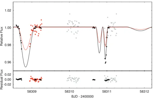
The orbital and astrophysical parameters obtained from the joint photodynamical analyses are given in Table4. The corresponding model light curves for different sections of the observed lighcurves are presented in Figs 4,5, and6, while the RV-curve portion of the solution was shown previously in Fig.3. Finally, the model ETV curve plotted against the observed ETVs is shown in Fig.7.

8 D I S C U S S I O N O F T H E R E S U LT S 8.1 Astrophysical properties

Our photodynamical analysis of the available data for EPIC 249432662, the ‘great eclipser’, has led to a reasonably well- constrained set of system parameters (see Table4). Among these are the masses of the three constituent stars, which are determined well enough to make a contribution to the collection of empiri- cally well-measured radii and masses of stars on the lower main sequence. We plot theR(M) points for the three stars in the ‘great eclipser’, with error bars in Fig.8. Also shown in the figure are two sets of theoretical stellar models, as well as a number of well- measured stars in binary systems. We can see that the three great eclipser stars lie somewhat above the stellar model locations, but comfortably in among the collection of other well-measured stars in binary systems. The usual explanation for the somewhat larger radii of the measured systems is thermal ‘inflation’ due to interactions in the binary system, e.g. tidal heating (see e. g. Han et al.2017, and references therein).

A fundamental check on the system parameters that we have found can be made by computing the photometric parallax for the target, and then comparing it to the Gaia distance. To obtain this quantity using our photodynamically determined stellar radii and temperatures, we calculate the bolometric luminosities and, thereby, the absolute bolometric magnitude of each star. Then, these values are converted into absolute visual magnitudes via the formulae of Flower (1996) and Torres (2010). Finally we compute the net absolute visual magnitude for the system as a whole, and obtainMV= 6.57±0.14. We then utilized a web-based applet¹²to estimateE(B

11The details of the initialization of the numerical integrator for quasi- synchronous rotation, taking into account even the likely orbital plane and stellar spin precession in the case of an inclined triple system, are described in Appendix A

12http://argonaut.skymaps.info/query?