Eclipse timing variation analysis of OGLE-IV eclipsing binaries towards the Galactic Bulge – I. Hierarchical triple system candidates

(1)

Eclipse timing variation analysis of OGLE-IV eclipsing binaries towards the Galactic Bulge – I. Hierarchical triple system candidates

T. Hajdu,

^1,2,3,4^‹

T. Borkovits ,

^3,5

E. Forg´acs-Dajka ,

¹

J. Sztakovics,

^1,6

G. Marschalk´o

^1,3,5

and G. Kutrov´atz

¹

1Department of Astronomy, Eötvös Loránd University, Pázmány Péter stny. 1/A, H-1118 Budapest, Hungary

2Konkoly Observatory, Research Centre for Astronomy and Earth Sciences, Hungarian Academy of Sciences, Konkoly Thege Mikl ´os ´ut 15-17, H-1121 Budapest, Hungary

3Wigner Research Centre for Physics of HAS, PO Box 49, H-1525 Budapest, Hungary

4MTA CSFK Lendület Near-Field Cosmology Research Group, Konkoly Thege Miklós út 15-17, H-1121 Budapest, Hungary

5Baja Astronomical Observatory of Szeged University, Szegedi ´ut, Kt. 766, H-6500 Baja, Hungary

6Department of Physics, Eszterházy Károly University, H-3300 Eszterházy tér 1 Eger, Hungary

Accepted 2019 February 26. Received 2019 February 26; in original form 2019 January 25

A B S T R A C T

We report a study of the eclipse timing variation (ETV) of short period (P1 ≤ 6^d) eclipsing binaries (EBs) monitored during the photometric surveyoptical gravitational lensing experiment-IV. From the 425 193 EBs, we selected approximately 80 000 binaries that we found suitable for further examination. Among them, we identified 992 potential hierarchical triple (or multiple) system candidates exhibiting light-travel time effect (LTTE). Besides, we obtained the orbital parameters of these systems and carried out statistical analyses on the properties of these candidates. We found that (i) there is a significant lack of triple systems where the outer period is less than 500 d, (ii) the distribution of the outer eccentricities has a maximum around e2 ≈ 0.3, and (iii) the outer mass ratio calculated from an estimated minimum mass of the third component is lower thanq2∼0.5 for the majority of the sample.

We also present some systems that deserve special attention: (i) There are four candidates that show double periodic ETV, which we explain by the presence of a fourth companion; (ii) For two systems, the perturbations of the third component are also found to be significant therefore we give a combined dynamical and LTTE ETV solution; and (iii) For one system, the third component is found to be probably in the substellar mass domain.

Key words: methods: numerical – binaries: close – binaries: eclipsing.

1 I N T R O D U C T I O N

The study of variable stars has a long history going back to antiquity (Jetsu et al.2013). The recent boom of the discovery of thousands of new variable stars is a natural by-product of the large stellar surveys such as, e.g. NASA’sKeplerMission (Prˇsa et al.2011) and optical gravitational lensing experiment (OGLE; Soszy´nski et al.2016).

The investigation of triple stellar systems plays a significant role not only in the understanding of the orbital evolution of close binaries, but also in the study of their whole life (from their formation to the death of the binary components; Toonen, Hamers &

Portegies Zwart2016). Furthermore, the various formation theories of close binary systems, e.g. the so-called Kozai cycles with tidal friction mechanism (see e.g. Kiseleva, Eggleton & Mikkola1998;

Fabrycky & Tremaine2007; Naoz & Fabrycky2014), as well as the

E-mail:t.hajdu@astro.elte.hu

recently proposed different disc and core fragmentation procedures (Moe & Kratter2018; Tokovinin2018), require the presence of an additional, third stellar component for the explanation of the large number of the shortest (less than a few days) period, non-evolved binary stars.

One of the best known methods for the identification of a third companion around an eclipsing binary (EB) is based on the detection and analysis of the eclipse timing variations (ETVs) of the binary.

If an EB has a distant, third companion, its distance from the observer varies periodically due to the EB’s revolution around the common centre of mass of the triple (or multiple) system. As a natural consequence, the light-travel time effect (LTTE) occurs, which manifests in periodic fluctuations in the observed times of the eclipses. Such kind of periodic ETVs has been found in hundreds of EBs in the last 60–70 yr.

Several surveys have provided excellent photometry for ETV analysis. Besides the investigations of ultraprecise space photometry such as Kepler(Rappaport et al.2013; Conroy et al.2014;

Downloaded from https://academic.oup.com/mnras/article-abstract/485/2/2562/5366746 by guest on 29 April 2019

(2)

Borkovits et al.2015,2016) andCoRoT(Hajdu et al.2017), there are several studies that used ground-based survey data for searching multiple stellar systems, see e.g. Li et al. (2018).

TheOGLEwas designed for discovering dark matter using the microlensing technique in 1992 (Udalski et al.1992). Observations of the currently running projectOGLE-IVare made at Las Campanas Observatory, Chile with the 1.3 m Warsaw Telescope, which is currently equipped with a mosaic CCD camera. The majority of the observations were carried out in CousinsIphotometric band with an exposure time of 100 s, while a much smaller part of them were made in JohnsonVband with the exposure time of 150 s. Recent and past OGLE surveys were found to be useful, e.g. for exoplanet exploration (Bouchy et al.2004) and for the investigation of variable stars (Soszy´nski et al.2016).

The Galactic Bulge part of the OGLE-IV survey with its approximately half million EBs, which were identified by Soszy´nski et al. (2016), gives us a good chance to increase the number of the candidates of hierarchical triple stellar systems. The authors also mentioned some potential triple systems in their paper that were also found by our algorithm.

Recently, Zasche et al. (2016) and Zasche, Wolf & Vraˇstil (2017) investigated light curves (LCs) of theOGLELarge and the Small Magellanic Cloud eclipsing binaries (EBs) and found some additional components and determined their orbit.

In this paper, we are searching for hierarchical triple star candidates towards the Galactic Bulge with the analysis of ETVs of EBs observed during theOGLE-IVsurvey. For this study, we use publicly availableOGLE- IVphotometric data¹(Soszy´nski et al.

2016).

In Section 2, we shortly formulate the mathematical background of the third body affected ETV analysis.

In Section 3, we outline the steps of our investigation, starting with the methods used for data acquisition and automatic O− Ccurve generation, then continuing with the system selection and, finally, closing with a short description of some details of the applied ETV and the auxiliary light curve analyses as well.

The results of the analysis of the ETVs of the new hierarchical triple candidates, as well as some other interesting by-products of our research, are discussed in Section 4.

Finally, a short summary is given in Section 5.

2 E F F E C T S O F A T H I R D B O DY O N T H E E T V In this paper, we define ETV as the difference between the observed and calculated times of minima (which is also called asO−C):

=T(E)−T0−PsE, (1)

whereT(E) denotes the time of theEth eclipse,T0=T(0) is the time of the ’zeroth’ eclipse, andPsdenotes the orbital period of the binary. Our basic model is given by

= 2

i=0

ciEⁱ+

LTTE+dyn

E

0. (2)

The constant and linear terms of the polynomial inEgive corrections toT0andPs. The second-order coefficient provides the half rate of the linear variation in period. Note that this term had significant value only in a few cases. These systems are marked in the corresponding tables. The second and third components in the right- hand side of the equation,LTTEanddyn, refer to the contributions

1ftp://ftp.astrouw.edu.pl/ogle/ogle4/OCVS/blg/ecl/phot ogle4/

of LTTE and short time-scale dynamical third-body perturbations.

Note that an ETV and therefore equation (2) may contain additional components, for example, the effect of the apsidal motion in an eccentric EB. However, the vast majority of the short period EBs in our sample revolve on circular orbit and therefore this component does not play any role.

In the following two subsections, we describe shortly the LTTE and dynamical terms.

2.1 The light-travel time effect

According to our knowledge, Chandler (1888) was the first to mention LTTE as a possible origin of the observed ETVs of Algol.

Later, the widely used mathematical description of an LTTE forced ETV was published by Irwin (1952). He also gave a graphical fitting procedure for determining the elements of the light time orbit from the ETVs that had been investigated by the use of the eclipse timing diagrams. Traditionally, these diagrams were calledO–Cdiagrams (see e.g. Sterken2005for a short review on the advantages ofO–C diagrams in the analyses of period variations).

There are several other mechanisms capable of producing ETVs in EBs, and some of them may even strongly mimic LTTE-like behaviour. Therefore, the detection of the third component with this method is not an easy matter. In this regard, Frieboes-Conde &

Herczeg (1973) listed four criteria that an ETV curve should fulfil for an LTTE solution. These criteria can be summarized as follows:

(1) The shape of the ETV curve must follow the analytical form of an LTTE solution. (2) The ETVs of the primary and secondary minima must be consistent in both amplitude and phase with each other. (3) The estimated mass or the minimum mass of the third component, derived from the amplitude of the LTTE solution, must be in accord with photometric measurements or limits on third light in the system. (4) Variation of the systemic radial velocity (if it is available) should be consistent with the LTTE solution.

According to Irwin (1952), the LTTE contribution takes the following form:

LTTE= −aABsini2

c

1−e²₂

sin (v2+ω2) 1+e2cosv2

, (3)

whereaABdenotes the semimajor axis of the EB’s centre of mass around the centre of mass of the triple system, whilei2,e2, andω2

stand for the inclination, eccentricity, and argument of periastron of the relative outer orbit, respectively. Furthermore,cis the speed of light andv2is the true anomaly of the third component. Note the negative sign on the right-hand side, which arises from the use of thecompanion’sargument of periastron, instead of the argument of periastron of the light time orbit of the EB (ωAB=ω2+π).

The amplitude of the LTTE takes the form ALTTE= aABsini2

c

1−e₂²cos²ω2, (4)

while the mass function f(mC), analogous to its spectroscopic counterpart for single-line spectroscopic binaries, is usually defined as

f(mC)= m³_Csin³i2

m²_ABC = 4π²a_AB³ sin³i2

GP₂² , (5)

and can be calculated from the parameters of the LTTE solution.

Using the mass function, the amplitude of the LTTE can be approximated as

ALTTE≈1.1×10⁻⁴f(mC)^1/3P₂^2/3

1−e²₂cos²ω2, (6)

(3)

wheref(mC) should be expressed in solar masses,P2in days, and ALTTEis also resulted in days.

Note that if the mass of the EB is known, the minimum mass (i2=90 deg) of the third component can be determined based on the mass function (f(mC)).

2.2 Dynamical perturbation of the third component on the ETV

In tight hierarchical triple stellar systems, the short time-scale three- body perturbations on the Keplerian two-body motion of the inner binary may also alter the ETVs significantly. This dynamical ETV contribution was analytically described in a series of papers by Borkovits et al. (2003,2011,2015).

The dynamical ETV component (dyn) has a complex depen- dence on the orbital elements of the inner and outer orbits, and their relative configurations as well. Furthermore, for eccentric inner orbits even the orbits’ relative orientation to the observer becomes an additional important factor. A comprehensive description of these effects can be found in Borkovits et al. (2015). In our sample, however, we calculate dynamical effects only for circular EBs.

Therefore, for our purposes it is satisfactory to use the substantially simpler formula of Borkovits et al. (2003) that takes the following form:

dyn=Adyn 1−3 2sin²im

M+ 3

4sin²imS

, (7)

where

M=v2−l2+e2sinv2, (8)

S =sin(2v2+2g2)+e2

×

sin(v2+2g2)+1

3sin(3v2+2g2)

(9) stand for the time-dependent functions of the true anomaly (v2) as well as the mean anomaly (l2) of the outer body on its relative orbit around the EB’s centre of mass, whileg2is the tertiary’s argument of periastron measured from the intersection of the inner and outer orbital planes. Furthermore,imdenotes the mutual (relative) inclination of the inner and outer orbits, while the mass and period ratios of the inner and outer subsystems occur in the amplitude-like quantity:

Adyn= 1 2π

mC

mABC

P₁² P2

1−e²₂−3/2

. (10)

Note that despite the fact that the true magnitude of the dynamical ETV can be significantly altered by the two eccentricities and the mutual inclination as well (Borkovits et al.2011), it was found by Borkovits et al. (2016) that in most casesAdyngives a reasonable estimation at least for the magnitude of the short-term dynamical ETV contribution.

In this paper, we present two short periodic hierarchical triple stellar system candidates with significant dynamical contribution (see Section 4.1).

3 B A S I C S T E P S O F T H E A N A LY S I S 3.1 System selection

TheOGLE-IVsurvey provided around 425 193 light curves of EBs that were observed inIandVbands. Since theIband light curves

typically contain much more points thanV band ones, we relied only on the former photometric band data for our analysis. Our main goal was to find hierarchical triple stellar candidates whose outer period (P2) is shorter than, or comparable to, the length of the observations. Unfortunately, most of the data trains do not contain enough data points (more than the half of the cases contain less than 1000 points) for a detailed examination. Therefore, we investigated only those systems whose light curves contain more than 4000 points. Applying this criterion, we reduced our sample from the original 425 193 EBs to∼80 000 systems.

3.2 Determination of times of minima

To determine the times of minima, we used a slightly modified version of the algorithm used by Hajdu et al. (2017). Note that a similar algorithm was used by Burggraaff et al. (2018).

For the determination of the minima times, we used phase-folded and binned light curves of the systems. The initial periods for the phase-folding processes were taken from the original OGLE site. In some cases, these periods were updated and then the phase-folding was reiterated by the use of the period corrections obtained from the ETV analyses.

The folded light curves were binned into 1000 equally spaced phase cells, according to the orbital phases of each measured points.

Then, the weighted arithmetic mean magnitudes were calculated cell by cell, and associated with the phase of the cell mid-points. (For the weighting, the uncertainties of each individual data points were used). In the next step, we formed 12th order polynomial template functions for the primary and secondary eclipses of the folded and binned light curves. We intended to use these templates to determine the mid-times of the individual eclipse events.

Unfortunately, in most cases the individual cycle to cycle light curves are badly covered and therefore we were not able to determine individual times of minima with the necessary accuracy. Thus, we decided to use normal minima. After some attempts, we came to the conclusion that calculating one normal minimum for every 17 consecutive binary cycles would provide the best compromise between the requested phase coverage of any individual eclipsing minima, and the decreasing time-resolution, and smoothing of the ETVs.

We found that using the templates of the two types of eclipses at once we can reduce the uncertainties of the ETV data. In our work, we used these ETVs for analyses, but we also used the primary and the secondary ETVs for confirmations. Note that this dual fit process is applicable only if the eccentricity of the inner orbit is zero, so there is no apsidal motion.

3.3 ETV analysis

To select those systems that exhibit periodic ETVs, we applied a Levenberg–Marquardt (LM)-based process fitting a sine function together with a second-order polynomial in the following form:

f(x)=a0+a1·x+a2·x²+a3·sin a4+2π a5

·x

. (11) The initial period (a5) was varied between 80×P1and 4000 d with a step size of 10×P1, and the best fit was chosen viaχ²search.

The former value was found to be an appropriate lower limit for reasonable outer periods, while the latter one is twice the maximum length of the data series.

Then, with the use of a combined grid search and LM method our code searches for an LTTE solution (equation 3) together with

(4)

Table 1. LTTE solutions for the 258 most certain hierarchical triple star candidates of the OGLE IV sample (the full table can be obtained in machine-readable form in the electronic edition of the paper).

ID T0 P1 P2 aAB·sin (i2) e2 ω2 τ2 f(mC) P1

(HJD-2450000 d) (d) (d) (R⁾ ^(deg) ^(d) ^[×10⁻¹⁰^d^c^]

28238 5265.711315 0.336880 424.5±9.0 123.9±10.7 0.61±0.10 31.7±0.9 5606.1±9.3 0.1413±0.03339 – 32148 5265.437046 0.311293 762.5±425.4 143.8±100.3 0.41±0.40 239.9±4.2 5484.1±329.2 0.0685±0.21020 – 35547 5265.221608 1.745663 648.3±36.0 151.8±8.1 0.43±0.13 75.7±1.6 5965.1±21.4 0.1116±0.03050 – 47614 5265.569008 0.290397 1406.0±7.7 142.3±5.3 0.53±0.04 10.3±0.3 6026.3±10.3 0.0196±0.00178 – 117862 5260.079711 1.048052 438.1±13.7 101.9±5.3 0.05±0.11 157.0±11.6 5458.2±105.9 0.0740±0.01464 – 118172 5260.619707 0.289513 859.7±211.1 28.5±4.1 0.20±0.42 93.3±7.0 5743.9±164.1 0.0004±0.00041 – 118178 5260.599311 0.330831 772.0±55.6 70.1±3.9 0.24±0.18 49.7±4.6 5578.7±71.7 0.0077±0.00252 32.4±5.7 ...

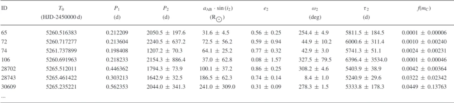
Table 2. LTTE solutions for the remaining, less certain hierarchical triple star candidates of the OGLE- IV sample (the full table can be obtained in machine-readable form in the electronic edition of the paper).

ID T0 P1 P2 aAB·sin (i2) e2 ω2 τ2 f(mC)

(HJD-2450000 d) (d) (d) (R⁾ ^(deg) ^(d)

65 5260.516383 0.212209 2050.5±197.6 31.6±4.5 0.56±0.25 254.4±4.9 5811.5±184.5 0.0001±0.00006

72 5260.717277 0.213604 2240.5±637.2 72.5±56.2 0.59±0.94 44.9±10.2 6000.6±311.4 0.0010±0.00240

74 5261.737899 0.198408 1207.2±70.3 64.1±25.2 0.77±0.32 42.9±3.0 5741.3±51.1 0.0024±0.00231

106 5260.691963 0.218233 2154.3±886.4 37.0±62.8 0.08±1.57 327.5±79.5 6396.4±3534.0 0.0001±0.00046 28702 5265.512011 0.446362 1794.3±73.9 100.1±37.2 0.86±0.25 308.2±4.6 5403.9±38.9 0.0042±0.00364 28743 5265.461422 0.303213 1642.9±32.5 186.5±62.3 0.74±0.14 8.4±1.0 5240.9±29.6 0.0322±0.02342 30609 5265.235221 0.562353 2044.0±341.3 241.0±309.0 0.31±0.09 278.3±1.5 5333.8±178.3 0.0449±0.13763 ...

the parabolic term. For this process, the initial values of some of the parameters (third-body period, polynomial coefficients) are taken from the previous, sine fit.

To get the best-fitting ETV solution, the initial values of the eccentricity (e2), argument of the periastron (ω2), and periastron passage time (τ2) were set to 4–6 different, evenly spaced values within their physically realistic range.

Then, in the last stage, the goodness of the solutions was tested and therefore the selection of the triple candidate systems was carried out also in an automatic manner. The first criterion was that the amplitude (ALTTE) of the LTTE solution (equation 4) has to be higher than one and the half times the average absolute difference between successiveO−Cpoints. The other criterion was based on the normalizedχ²value that was counted in the following form:

χ²= 1 N

N i=1

(yi−fi)²

σ_i² , (12)

where N is the number of theO−Cpoints,yiis the value of the ithO−Cpoint,firepresents theithO−Cvalue derived from the ETV solution, and finallyσiis the uncertainty of theith O− C point. Finally, this list was corrected (basically reduced) through a manual inspection.

4 R E S U LT S

In conclusion, we have found 992 potential hierarchical multiple stellar system candidates in the photometric data of theOGLE-IV survey. We divided these candidates into two groups. In the first group of the more probable triples, we put basically those systems for which the outer period is less than 1500 d and the amplitude is at least three times higher than the variance of the residual, or else the period is lower than 1000 d, while the other group contains the remaining, less confident cases.

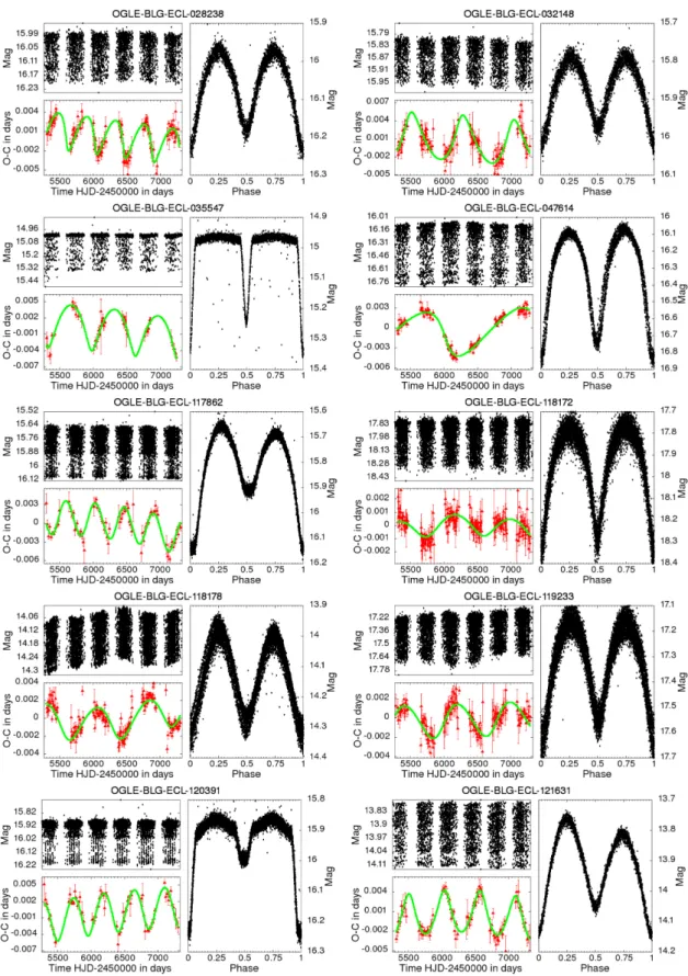
The results obtained for the two sets of our candidates are listed in Tables1and2, respectively. These tables provide the OGLE ID, the epoch (T0), the inner and outer periods (P1,P2), the eccentricity (e2), argument of the periastron (ω2) and periastron passage time (τ2) of the third companion, the projected semimajor axis of the light- time orbit (aABsini2), the mass function (f(mC)), and the parabolic term (P1) where it is significant. Furthermore, we plot the ETVs together with the LTTE solutions and the raw and folded light curves in Fig.1as well.

In what follows, after enumerating some individual systems with special interests (Sects. 4.1, 4.2, 4.3) we carry out detailed statistical analyses of the properties of our candidates in Section 4.4.

4.1 Systems with significant dynamical effect

For the vast majority of the investigated systems, in comparison to the LTTE term, the dynamical contribution to the ETV can safely be ignored. This fact was far not unexpected, as the amplitude of the dynamical ETV is scaled with the EB’s period, hence our sample systems with their typical period ofP1<1 d are strongly unfavourable for the detection of such effect. Despite this, we detected two systems where the results of the preliminary LTTE analysis have predicted significant dynamical ETV contribution.

For these two systems, in theory, we were able to determine system masses, though only with large uncertainties. The parameters of these systems are tabulated in Table3and the LTTE+dynamical ETV solutions are presented in Figs2and3.

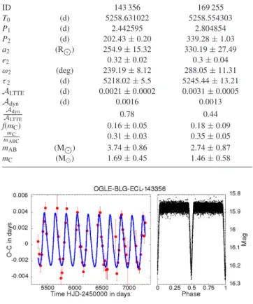
OGLE-BLG-ECL-143356is an Algol-type EB with a period of P1∼2.^d4 and moderately different primary and secondary eclipse depths (see Fig.2; right-hand panel). The amplitude of the dynamical effect is∼80 per cent of LTTE amplitude. Our results imply that the system is formed by three stars more massive than our Sun. The total mass of the inner binary was found to be∼3.7±0.9 M, while

(5)

Figure 1. The rawI-band (upper left-hand panel) and the folded (right-hand panel) light curve and the ETV data together with the LTTE solution (lower left-hand panel) for the 255 most certain candidate systems. (The full figure for all the triples can be obtained in the electronic edition of the paper.).

(6)

Table 3. Orbital elements from combined dynamical and LTTE solutions.

ID 143 356 169 255

T0 (d) 5258.631022 5258.554303

P1 (d) 2.442595 2.804854

P2 (d) 202.43±0.20 339.28±1.03

a2 (R⁾ ^254.9^±^15.32 ^330.19^±^27.49

e2 0.32±0.02 0.3±0.04

ω2 (deg) 239.19±8.12 288.05±11.31

τ2 (d) 5218.02±5.5 5245.44±13.21

ALTTE (d) 0.0021±0.0002 0.0031±0.0005

Adyn (d) 0.0016 0.0013

Adyn

ALTTE 0.78 0.44

f(mC) 0.16±0.05 0.18±0.09

m_C

m_ABC 0.31±0.03 0.35±0.05

mAB (M⁾ ^3.74^±^0.86 ^2.74^±^0.87

mC (M) 1.69±0.45 1.46±0.58

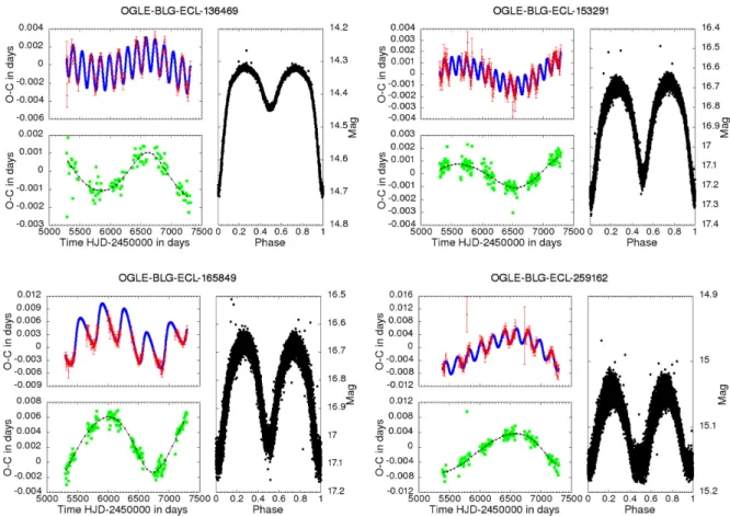
Figure 2. ETV of OGLE-BLG-ECL-143356 (red) together with the LTTE+dynamical ETV solution (blue) in the left-hand panel. The folded light curve in the right-hand panel.

Figure 3. ETV of the system OGLE-BLG-ECL-169255 (red) together with the LTTE+dynamical ETV solution (blue) in the left-hand panel. The folded light curve in the right-hand panel.

the mass of the third component was found to be∼1.7±0.5 M. Furthermore, the folded light curve suggests that the inner binary is formed by two similar stars and therefore the whole triple might be made up of components of almost equal masses.

OGLE-BLG-ECL-169255is an another Algol-type EB with un- equally bright components (see Fig.3; right-hand panel). According to our solution, the third component has a mass of∼1.5±0.6 M. Note that the amplitude of the dynamical delay is less than the half of the amplitude of the LTTE.

4.2 Systems with double periodic ETVs

We found four systems where the ETV analyses suggest double periodic solutions. Similar to the investigation of Zasche et al.

(2017) about OGLE-SMC-ECL-4024, we interpret these ETVs as manifestations of two independent LTTEs occurring in (dynamically) non-interacting (2+1)+1 hierarchical-type quadruple stellar systems.

Therefore, we fit a double LTTE solution (via LM) with some appropriate initial guesses. The results of our process are plotted in Fig. 4and the orbital parameters are shown in Table4. The parameters for the middle orbit are in the upper part of the table, while the bottom part contains the parameters of the outer LTTE solution.

Note that our model neglects the dynamical effects therefore the computed orbital parameters are only indicative. This is especially true in the case of OGLE-BLG-ECL-165849 where the ratio of the outer periods is small (P3/P2 < 6), which might indicate strong dynamical effects or instability particularly regarding these orbital parameters (e2 ∼ 0.46). Further complex examinations are required to understand the true nature of these systems.

While OGLE-BLG-ECL-136469 shows a β Lyrae-type light variation, the other three short period (P1<0.4 d) EBs seem to be typical W UMa-type stars with small differences between the depths of the primary and secondary eclipses. There is a possibility that the fourth components have also significant effect on the evolution of the short periodic binaries and triples as well.

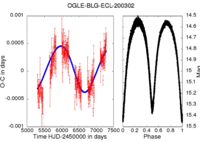
4.3 System with possible substellar companion

OGLE-BLG-ECL-200302is a short-periodic (P1=0.24^d) W UMa- type EB for which our ETV solution (Fig.5) gives a very low value of the mass function (f(mC) =0.00002 ±0.00003). In order to estimate the minimum mass of the third component, we calculated the total mass of the binary by applying the empirical period–

mass relation of short periodic binaries (Dimitrov & Kjurkchieva 2015). Such a way we got mAB=1.29 M. In this way, the minimum mass of the third companion is found to be mCmin= 0.034±0.044 M, which is in the substellar domain. The mass of the tertiary will remain in the substellar domain if 28 deg≤i2≤ 152 deg therefore we can conclude that this is most likely a brown dwarf.

4.4 Statistical analysis

Due to the large number of triple system candidates, it is worth- while to examine distributions of several parameters that can be determined using only the LTTE delays. These parameters are the periods (P1 and P2), the outer eccentricitye2, and the mass function f(mC). These parameters are available for all systems (see Tables 1 for the 258 chosen systems and 2 for all the rest).

In spite of the huge amount of potential hierarchical candidates we found, the relatively high uncertainty of parameters suggested that we focus our statistical investigation on those systems where the determinable parameters have lower uncertainty. For the sake of completeness, we also present the distributions of the same parameters for the extended sample of all the candidate systems.

4.4.1 Outer eccentricity

Due to the relatively high uncertainty of our results, similar to Murphy et al. (2018), we use the kernel density estimation

(7)

Figure 4. Hierarchical four body candidates with double LTTE solution (the blue line in the upper left-hand panel) and the residual of the short periodic solution (the green squares in the bottom left-hand panel). Here, the black dotted lines show the LTTE solution of the third orbit. The folded light curve of the system is in the right-hand panel.

Table 4. Results of double LTTE solution fit.

ID T0 P1 P2 a·sin (i2) e2 ω2 τ2 f(mC)

(d) (HJD-2450000 d) (d) (R⁾ ^(deg) ^(d)

136469c 5260.409845 0.681115 149.23±0.16 69.97±1.87 0.08±0.05 112.46±37.97 5327.52±15.85 1.3128±0.075 153291c 5260.916183 0.283085 120.06±0.15 31.42±1.32 0.28±0.07 178.47±14.21 5357.23±5.04 0.5764±0.051 165849c 5260.553794 0.276678 367.34±0.54 182.57±22.72 0.46±0.05 178.46±34.77 5469.94±9.06 2.2016±0.558 259162c 5376.300087 0.355920 192.53±0.54 83.40±3.71 0.15±0.08 3.80±32.75 5296.71±18.00 1.3231±0.129

ID P3 a·sin (i3) e3 ω3 τ3 f(mD)

(d) (R⁾ ^(deg) ^(d)

136469d 1633.45±115.30 45.26±3.25 0.23±0.12 265.78±33.36 5853.13±226.57 0.1283±0.046

153291d 2077.10±339.21 46.27±7.29 0.16±0.07 101.71±61.23 6645.60±947.48 0.1111±0.089

165849d 2026.46±298.60 203.77±37.09 0.3±0.05 45.25±12.70 6601.04±636.86 0.5666±0.457

259162d 2036.21±224.98 188.41±17.37 0.30±0.09 23.88±21.56 5103.95±485.25 0.5152±0.266

method to determine its dispersion. This takes the functional form

f(e)= 1 N

N i=1

K(e, ei, σi), (13)

where

K(e, ei, σi)= 1 σi

√2πexp −(e−ei)² 2σ_i²

(14) is the kernel function, while ei and σi are the ith measured eccentricity and its uncertainty.

Fig.6shows that the distribution has a significant peak around e2≈ 0.3, which is consistent with the results of Borkovits et al.

(2016). Including all systems, we got a slightly highere2≈ 0.4 value. This slight increase in the eccentricity as a function of the period can also be observed in the case of wide binary systems (see e.g. Tokovinin & Kiyaeva2016).

As one can see in Fig.7,the cumulative distribution is inconsistent both with the ’thermal’ distribution that would be linearly rising withe2(originally posited by Jeans1919) and also with the uniform (flat) distribution. Similar to binary systems reviewed in Duchˆene &

Kraus (2013), none of the ‘thermal’ and ‘flat’ curves represent the true outer eccentricity distribution of our sampled triples.

(8)

Figure 5. ETV ofOGLE-BLG-ECL-200302and the LTTE solution (the blue line) that suggests the presence of a substellar third body companion (left-hand panel). Folded and binned light curve of the system is in the right-hand panel.

Figure 6. Distribution of outer eccentricity (e2) of the selected systems (yellow) have a peak arounde2∼0.3. For the extended sample of all the candidate systems (blue), the peak value is shifted towards slightly higher eccentricities.

4.4.2 Tertiary period

In Fig.8, we present the distribution of the outer orbital periods of the 258 selected systems (yellow) and those systems from the full list whereP2is lower than 2000^d(blue). This histogram shows a flat maximum betweenP2≈500–800^d, which lower limit may be explained by observational selection effects. Furthermore, in general, the shorter the outer period the lower the LTTE amplitude (equation 6), which acts against the detection of the lowest outer period third companions. The number of candidates is rising with the outer period. The significant peak aroundP2∼1500^dmay come from the fitting procedure as it is more likely to converge to this value if the period (P2) is longer than the observation.

Fig.9shows the correlation plot of the outer versus inner periods.

Besides our triple candidates, for comparison we plot also the locations of hundreds of other hierarchical triples, most of those discovered in the primeKeplerfield. For better clarity, the blue lines denote the limits of the regions where the amplitudes of the LTTE (ALTTEand dynamicalAdyn) effects are likely to exceed 50 s, a value that roughly approximates the threshold of the probable detection of

Figure 7. Cumulative distribution of the outer eccentricities (e2) of our selected 258 triple candidates (black), all of our triple candidates (cyan), and 222Keplertriple candidates of Borkovits et al. (2016) (red), respectively.

The green curve, shown for comparison, represents the cumulative distribution expected for a uniformly distributed set of eccentricities between zero and 1. The blue curve is for an eccentricity distribution that increases linearly withe2. None of the comparison curves give a good match with the observed distribution, which results from the distribution of the eccentricity having a peak betweene2=0.2 ande2=0.4. For comparison to the eccentricities of unperturbed wide field binaries in the same period regime, see (Duchˆene &

Kraus2013).

Figure 8. Distribution of the outer orbital periods (P2) from LTTE solution for the sample of the 258 most certain (yellow) as well as for all (blue) candidate triple systems whose period is lower than 2000 d.

an ETV. In this figure, the vast majority of our candidate systems are located in a well-defined area that is mainly dominated by LTTE.

The centre of the group is really close to the observation length (∼2000^d), perhaps because the reliability of our LTTE searching algorithm decreases if the outer orbital period becomes longer than the time span of the data. Another possibility is that if the real period is significantly longer than our data length then the LM fit more likely converges to a lower period value that is closer to the duration of the time span.

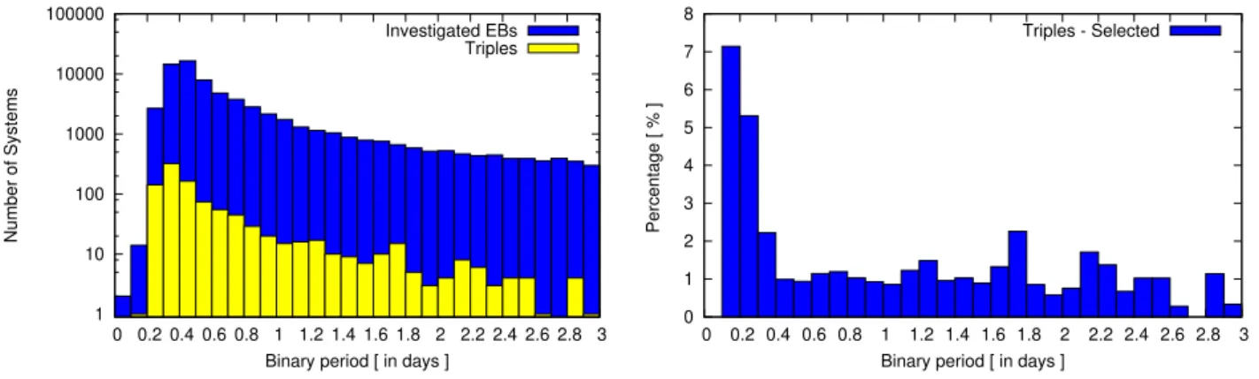
4.4.3 Frequency of triple systems

We compare the period distributions of the investigated 78 912 EBs and the detected triple system candidates in the left-hand panel of Fig. 10. A significant peak occurs around P1 = 0.4^din both cases. The lack ofP1<0.2^dperiod systems is consistent with the

(9)

Figure 9. The location of the 992 triple star candidates (the blue triangles) in theP1versusP2plane. For comparison, we plotted those short-period Kepler,K2andCoRoT-triple system candidates for which the inner and outer periods areP1≤20 andP2≤10 000 d. Following the work of Borkovits et al. (2016), the pure LTTE systems are marked with the black circles, while triples with combined LTTE+dynamical ETV solution are plotted with the green squares. The blue lines show the borders of the domains where the amplitudes of the LTTE and dynamical terms may exceed∼50 s, which can be regarded as a limit for an unambiguous detection. These limits were calculated for a hypothetical triple system of three, equally solar mass stars, with a typical outer eccentricity ofe2 =0.35, and quite arbitrarily,i2 = 60 deg andω2= ±90 deg. The shaded yellow area means that no LTTE can be detected, though dynamical effects may be significant and therefore certainly detectable. The purple region is a dynamically unstable region, in the sense of the stability criteria of Mardling & Aarseth (2001).

theoretical lower limit of the period of contact binaries (Rucinski 1992).

The right-hand panel represents the percentage of triples in relation to the investigated EBs. It is clearly visible that at lower periods the probability of the triplicity is significantly higher. This supports the idea that close binary systems need a third component for their formation, although the forming mechanisms might be various as noted in the introduction.

4.4.4 Minimum mass

In the absence of the true binary masses in our sample, the minimum masses were estimated from the mass function f(mC) with the assumption that mAB 2 M. We plot the distribution of the

Figure 11. Distribution of the minimum tertiary masses,mCminfor triple systems found inOGLE-IV. The tertiary masses are calculated from the LTTE solutions with the assumption ofmAB2M^.

Table 5. The seven systems where the third component has higher mass than the EB.

ID P1 P2 f(mC) mC

(d) (d) M

133 733 2.173444 746.1± 43.3 0.79±0.81 2.53±1.38 136 328 0.363304 1016.4± 10.8 0.70±0.05 2.38±0.09 150 450 5.646726 1807.2± 145.1 0.53±0.28 2.07±0.55 172 418 1.107474 1488.7± 39.4 0.90±0.34 2.71±0.56 209 134 0.436740 1298.1± 39.1 1.32±0.96 3.36±1.40 270 588 0.420899 834.4± 20.6 1.02±0.17 2.90±0.26 301 085 0.641771 4072.7± 33.8 0.86±0.66 2.64±1.10

predicted minimum masses of the third bodies in Fig.11. As far as we consider only the narrower sample of the most certain triples, we find a mostly flat distribution. There are seven candidate systems where the mass of the third component is higher than the mass of the EB. These systems are listed in Table5.

Regarding the total sample (blue), one can find that the vast majority of the candidate systems have minimum outer masses less than 1 M, i.e. an outer mass ratio ofq2min<0.5, which suggests that the third component in most cases is a lower mass object.

As shown in Fig.11, there is a lack of systems whosemCminis lower than 0.1 M. This may be either because the amplitudes of these systems are too low to detect with our method, or because they are actually uncommon. To decide the question, we examined the

Figure 10. Number of all EBs observed byOGLE-IV, the investigated EB systems, and found triple stellar systems as a function of the binaries’ orbital period (P1) in the left-hand panel. The right-hand panel shows the percentage of the triples in relation to the investigated EBs and the percentage of the investigated EBs in relation to all observed systems.

(10)

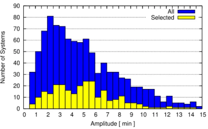
Figure 12. Distribution of the amplitudes from the LTTE solution for all systems (blue) and for the systems from the shorter list (yellow).

amplitude distribution of the candidates (see Fig.12). This suggests that we are able to find systems with amplitudes less than 1^m. Using equation (6) with the following parameters:mAB=2 M, mC = 0.1, andALTTE=1^m, we were able to estimate a minimum period necessary to detect such a small third component. It resulted in P2 = 1050^d, which is notably shorter than the used observation series. Based on this, we can conclude that substellar components in such EB systems are fairly rare.

4.4.5 Amplitude of the LTTE

Despite that we used ground-based photometry, for our research we identified a significant number of hierarchical triple stellar candidates with relatively low LTTE amplitudes (0.^m5≤ALTTE≤ 1.^m0). This is due to the fact that most of these systems have the deepest eclipse depths among our candidates, which increases the precision of the fitting method. Nevertheless, we have not identified any potential candidate with amplitude lower than half a minute. The distribution of the amplitudes of the LTTE solutions (see Fig. 12) shows gamma distribution with a maximum aroundALTTE≈2^m.

5 S U M M A RY A N D C O N C L U S I O N S

In this paper, we reported the results of our search for close, third stellar companions of EBs towards the Galactic Bulge derived from the photometric surveyOGLE-IVvia ETV. Owing to the long-term observations, we were able to find 992 third body candidates.

For four of them (OGLE-BLG-ECL-136469, OGLE-BLG- ECL-153291, OGLE-BLG-ECL-165849, and OGLE-BLG-ECL- 259162), we came to the conclusion that their ETVs can be well modelled with a double LTTE solution rather than a simple hierarchical stellar system solution. However, since our model neglects dynamic effects, the resulting parameters are only indicative.

We also found two systems with significant dynamical amplitudes (OGLE-BLG-ECL-143356 and OGLE-BLG-ECL-169255).

Furthermore, a potential substellar third component was also identified in systemOGLE-BLG-ECL-200302.

We investigated the orbital parameter distribution of our systems.

For the more reliable results, we selected 258 systems where the period and the eccentricity were estimated with lower uncertainties.

Besides, we also worked with the full list for comparison. Though we found a very strong peak in the distribution of the eccentricities neare2≈0.3, and for the full list a bit higher. The number of systems shows a strong increase with the rise of the outer period (P2).

Through our investigations, we found potential third components with relative high (∼1.8 M) and low (0.6 M) minimum masses even in the short-period case. We also determined our sensitivity limit for the selection that is around half a minute (ALTTE≈0.5^m).

There is a great deal of follow-up work that can be carried out in the future, such as the search for systems with apsidal motion. We also plan to investigate the interesting systems through light curve modelling.

AC K N OW L E D G E M E N T S

This project has partly been supported by the HAS Wigner RCP- GPU-Lab, the Hungarian National Research, Development, and Innovation Office, NKFIH-OTKA grants K-113117, K-115709, and KH-130372, and the Lend¨ulet Program of the Hungarian Academy of Sciences, project No. LP2018-7/2018. The authors are grateful to K. Perger and S. Pint´er for their valuable comments and suggestions.

We are also grateful for L. Dobos for his help in the numerical alignment especially withPYTHONfitting algorithms.

R E F E R E N C E S

Borkovits T., Érdi B., Forgács-Dajka E., Kovács T., 2003,A&A, 398, 1091 Borkovits T., Csizmadia S., Forgács-Dajka E., Hegedüs T., 2011,A&A, 528,

A53

Borkovits T., Rappaport S., Hajdu T., Sztakovics J., 2015,MNRAS, 448, 946

Borkovits T., Hajdu T., Sztakovics J., Rappaport S., Levine A., B´ır´o I. B., Klagyivik P., 2016,MNRAS, 455, 4136

Bouchy F., Pont F., Santos N. C., Melo C., Mayor M., Queloz D., Udry S., 2004,A&A, 421, L13

Burggraaff O. et al., 2018, A&A, 617, A32 Chandler S. C., 1888, Bull. Astron., 5, 499

Conroy K. E., Prˇsa A., Stassun K. G., Orosz J. A., Fabrycky D. C., Welsh W. F., 2014,AJ, 147, 45

Dimitrov D. P., Kjurkchieva D. P., 2015,MNRAS, 448, 2890 Duchˆene G., Kraus A., 2013,ARA&A, 51, 269

Fabrycky D., Tremaine S., 2007,ApJ, 669, 1298 Frieboes-Conde H., Herczeg T., 1973, A&AS, 12, 1

Hajdu T., Borkovits T., Forg´acs-Dajka E., Sztakovics J., Marschalk´o G., Benk"o J. M., Klagyivik P., Sallai M. J., 2017,MNRAS, 471, 1230 Irwin J. B., 1952,ApJ, 116, 211

Jeans J. H., 1919,MNRAS, 79, 408

Jetsu L., Porceddu S., Lyytinen J., Kajatkari P., Lehtinen J., Markkanen T., Toivari-Viitala J., 2013,ApJ, 773, 1

Kiseleva L. G., Eggleton P. P., Mikkola S., 1998,MNRAS, 300, 292 Li M. C. A. et al., 2018, MNRAS, 480, 4557

Mardling R. A., Aarseth S. J., 2001,MNRAS, 321, 398 Moe M., Kratter K. M., 2018,ApJ, 854, 44

Murphy S. J., Moe M., Kurtz D. W., Bedding T. R., Shibahashi H., Boffin H. M. J., 2018,MNRAS, 474, 4322

Naoz S., Fabrycky D. C., 2014,ApJ, 793, 137 Prˇsa A. et al., 2011,AJ, 141, 83

Rappaport S., Deck K., Levine A., Borkovits T., Carter J., El Mellah I., Sanchis-Ojeda R., Kalomeni B., 2013,ApJ, 768, 33

Rucinski S. M., 1992,AJ, 103, 960

Soszy´nski I. et al., 2016, Acta Astron., 66, 405

Sterken C., 2005, in Sterken C., ed., ASP Conf. Ser. Vol. 335, The Light- Time Effect in Astrophysics: Causes and cures of the O-C diagram.

Astron. Soc. Pac., San Fransisco, p. 3 Tokovinin A., 2018,AJ, 155, 160

Tokovinin A., Kiyaeva O., 2016,MNRAS, 456, 2070

Toonen S., Hamers A., Portegies Zwart S., 2016, Comput. Astrophys.

Cosmol., 3, 6

Udalski A., Szymanski M., Kaluzny J., Kubiak M., Mateo M., 1992, Acta Astron., 42, 253

(11)

Zasche P., Wolf M., Vraˇstil J., Pilarˇc´ık L., Juryˇsek J., 2016,A&A, 590, A85

Zasche P., Wolf M., Vraˇstil J., 2017,MNRAS, 472, 2241 S U P P O RT I N G I N F O R M AT I O N

Supplementary data are available atMNRASJonline.

Figure 1.The rawI band (upper left-hand panel) and the folded (right-hand panel) light curve and the ETV data together with the LTTE solution (lower left-hand panel) for the 255 most certain candidate systems.

Table 1.LTTE solutions for the 258 most certain hierarchical triple star candidates of the OGLE IV sample.

Table 2.LTTE solutions for the remaining, less certain hierarchical triple star candidates of the OGLE IV sample.

Please note: Oxford University Press is not responsible for the content or functionality of any supporting materials supplied by the authors. Any queries (other than missing material) should be directed to the corresponding author for the article.

This paper has been typeset from a TEX/L^ATEX file prepared by the author.