PARENTAL JOB LOSS, SECONDARY SCHOOL COMPLETION AND HOME ENVIRONMENT*

(1)

PARENTAL JOB LOSS, SECONDARY SCHOOL COMPLETION AND HOME ENVIRONMENT*

Tamás HAJDU – Gábor KERTESI – Gábor KÉZDI

(Received: 16 February 2018; revision received: 10 February 2019;

accepted: 15 April 2019)

This study examines the effect of parental job loss on adolescents’ school completion during the secondary school years and the moderating role of home environment in that effect. It uses rich survey data from Hungary on adolescents between 14 and 21 years of age, with detailed measures of parental employment and home environment. The study replicates the average negative effect found in the literature. No effect is found for families with a history of providing a cognitively stimulating home environment, but the negative effect is strong for other families. Home environment matters more than initial income in moderating the effect. The results highlight the protective nature of a cognitively stimulating home environment.

Keywords: job loss, home environment, school completion JEL classifi cation indices: J60, I20

* We thank Dániel Horn and István György Tóth as well as participants of the annual conference of Magyar Közgazdaságtudományi Egyesület (Hungarian Society of Economics) for their thought- ful comments. Melinda Tir provided excellent research assistantship.

This work was supported by the National Research, Development and Innovation Office of Hungary (Grant No. NKFI-116354) and the Horizon 2020 Twinning project EdEN (Grant No.

691676).

Tamás Hajdu, researcher at the Institute of Economics, Centre for Economic and Regional Studies of the Hungarian Academy of Sciences, Budapest. E-mail: hajdu.tamas@krtk.mta.hu

Gábor Kertesi, corresponding author. Researcher at the Institute of Economics, Centre for Eco- nomic and Regional Studies of the Hungarian Academy of Sciences, Budapest.

E-mail: kertesi.gabor@krtk.mta.hu

Gábor Kézdi, researcher at the Survey Research Center, University of Michigan and Institute of Economics, Centre for Economic and Regional Studies of the Hungarian Academy of Sciences, Budapest. E-mail: kezdi@umich.edu

(2)

1. INTRODUCTION

Job loss of parents is known to have negative effects on student outcomes in the US (Flanagan – Eccles 1993; Kalil – Ziol-Guest 2005, 2008; Kalil – Wightman 2011; Stevens – Schaller 2011; Johnson et al. 2012; Brand – Thomas 2014;

Hilger 2016), Canada (Coelli 2011), Norway (Rege et al. 2011), the UK (Gregg et al. 2012), as well as Hungary (Kertesi – Kézdi 2007). However, the negative average effect hides substantial heterogeneity, and this heterogeneity is not well understood .

Adverse economic conditions may reduce the opportunity costs of staying in school, thus reducing the dropout rate (Betts – McFarland 1995; Long 2015;

Adamopoulou – Tanzi 2017). They also increase financial distress for families that experience a job loss, thereby potentially leading to negative income effects on investment in education of their children (Becker – Tomes 1986; Coelli 2011), thus increasing the dropout rate. Overall results are not necessarily negative, they can be positive, as well. Goldin (1999) found that the Great Depression led to increases in school enrollment in the US. There are conflicting results on the moderating role of initial family income (Kalil – Wightman 2011; Stevens – Schaller 2011; Brand – Thomas 2014), as well.

Besides these human capital effects, parental job and income losses may lead to mental stress in the family (family conflict, divorce, erratic and disengaged behavior towards children) that hampers children’s cognitive and emotional development (McLoyd 1990; Conger – Elder 1994; Charles – Stephens 2004; Ananat et al. 2017), tending to decrease school achievement and increase dropout rate.

It is also known that children who grow up in better home environments and experience better parenting perform substantially better in school, even when com- paring families with the same income (Linver et al. 2002; Yeung et al. 2002; Davis- Kean 2005; Todd – Wolpin 2007; Kalil 2015). Joining these strands of literature we hypothesize that home environment moderates the effect of parental job loss on student outcomes: a history of a good home environment may provide protection against bad educational outcomes when economic distress hits a family.

We use rich longitudinal survey data to examine the heterogeneity of the effect of parental job loss by household income and home environment at the same time. We analyze the question in Hungary, a middle-income country where secondary education is predominantly financed by the state, and where over 90 per cent of the analyzed cohort completes some sort of secondary school. The data is especially well suited to analyze our research questions. It has monthly information on parental employment as well as detailed measures of family income and home environment, and the latter two are measured before the time of the potential job loss. The field period of the survey included the economic recession

(3)

of 2008–2010, thus inducing substantial variation in parental employment during the secondary school years of adolescents, even in families from the upper half of the income distribution and the home environment distribution.

First, we estimate the effect of parents experiencing a decline in employment (during secondary school years) on the probability that their child completes secondary school by age 21. Monthly employment data on parents allows us to differentiate large declines in the employment duration from smaller declines. We define a large decline as a 25 per cent or higher drop in the fraction of months employed in a regular job compared to the reference period averaged across the two parents. The effect of a large decline is a four percentage point decrease in the probability of completing secondary school by age 21, from a 93 per cent baseline probability. This is a strong association that amounts to a 50 per cent increase in the dropout probability. The association is of similar sign, but smaller for a small decline in parental employment. The estimated association is likely to be a causal effect, as supported by additional evidence of regressions with the pre-treatment outcomes. While we do not observe the source of job loss and thus cannot look at incidences of plant closures or other exogenous sources of variation, we control for a rich set of covariates and provide additional evidence that deliver a strong support for causal interpretation. Our identification strategy follows Stevens – Schaller (2011) and Coelli (2011).

Second, we show significant interaction of the effect with baseline household income and baseline home environment. Our measure of income takes into ac- count income, expenditures, home value and size, and the history of financial distress. Our measure of home environment is an adaptation of the cognitive stimulation subscale of the Home Observation Measurement of the Environment (HOME) inventory (designed for children between 10–14 years of age (Bradley et al. 2000)). We find a remarkably strong effect of parental job loss on adolescents in the lower half of the home environment distribution in non-poor families.

A large decline in parental employment leads to a 9 percentage point decline in the school completion rate, compared to a 93 per cent baseline completion probability in this group. The effect is smaller for adolescents in the lower part of the home environment distribution in poor families. We find virtually no effect in families from the upper half of the home environment distribution.

All of our results are conditional on a rich set of other covariates, and the results of “placebo” regressions with pre-treatment outcomes support their causal interpretation. They are also robust to alternative definitions of permanent income and alternative functional forms. The difference of the effect by home environment is strongest when home environment is measured by items related to parental investment in human capital (as opposed to measures that are closer proxies of permanent income or measures of behavior).

(4)

We consider two interpretations of our results that are not mutually exclusive.

First, families may be very different in their preferences toward investment in the human capital of their children. Parents with stronger preferences for such investment may keep up with their investment in children’s education even if they experience a large decline in their employment that leads to severe economic distress. Parents with weaker preferences may cut back on such investments that may lead to an increase in the propensity of their children to drop out of secondary school. Second, a history of a cognitively stimulating home environment may endow children with skills that help them maintain their educational outcomes even if their parents decrease the investment in their human capital due to the economic distress caused by job loss.

Our paper contributes to the literature in three ways. First, we use rich longitudinal data that allow us to examine the heterogeneity of the impacts by household income and home environment at the same time. Second, we compute parental job loss from the monthly employment history of the parents, which allows us to differentiate between large and small decrease in employment. Third, we analyze the data from a middle-income country, whereas the vast majority of the previ- ous papers concentrated on the rich developed countries (e.g. the US, the UK, Norway).

2. DATA AND METHOD

This study examines the effect of parental job loss on the completion of secondary school in Hungary. Primary and secondary school combined takes 12 years in Hungary; for most of the tracks this means 8 years of primary school and 4 years of secondary school, whereas for the most selective academic tracks the 12 years are split into 4+8 or 6+6 years between primary and secondary. For the cohorts in our sample education was compulsory until the age of 18. With the earliest school starting at the age of 6 and with no grades failed, students would turn 18 in their 12th grade. Compliance with the compulsory schooling age was far from perfect (Adamecz-Völgyi 2018).

We use data from the first six waves of the Hungarian Life Course Survey (HLCS). The HLCS is a panel survey that follows 10,000 students who were in the 8th grade in the spring of 2006. The survey sampled the 8th grade students who participated in the Hungarian National Assessment of Basic Competences (NABC), as well as the students with special needs who did not participate in the regular NABC but completed a simplified version of the reading comprehension test. Students with lower test scores and students with special needs are overrepre- sented in the sample, and we use sampling weights throughout the analysis to re-

(5)

store national representativeness. The first wave of the HLCS was conducted in the fall of 2006, when a typical respondent was 15 years old, and the sixth wave was conducted in the summer of 2012, when the typical respondent was 21 years old.

In this analysis we restrict the sample to the adolescents who participated in the sixth wave of the survey, had valid information on the employment of their parents through all survey waves, had their family unchanged¹, and were not early dropouts². Table A1 in the Appendix shows the number of observations and average values for important variables in the population represented by the HLCS, the baseline HLCS sample and the final sample through various steps of sample selection. Although attrition in the survey is non-negligible, the final sample is still broadly representative of the initial population in terms of test scores, parental education, parental employment and the affluence of their town of residence.

Our analysis examines the effect of parental job loss. Parental job loss is computed from the monthly employment history of the parents for the year preced- ing each interview, and indicates whether a parent was employed in a regular job, worked irregularly, was unemployed, or out of the labor force. We measure employment change as the change in the fraction of months employed in regular jobs between two time periods, September 2006 to August 2008 and September 2008 to August 2010. By coincidence, the recession of 2008 started around the time when dropping out of secondary school became a potential issue for the respondents of our survey: the modal respondent age was 17 in January 2009. We call the time period between September 2006 and August 2008 as the “before- recession period” and the September 2008 to August 2010 time period as the

“recession period”. Figure A1 in the Appendix shows that the unemployment rate of the population aged 35–59 (the parents’ generation) was around six per cent in the before-recession period and increased substantially in the recession period, reaching nine per cent by the end of our sample period.

Our main right-hand-side variables are two binary indicators: whether parental employment decreased to a large extent and whether parental employment decreased to a small extent (unchanged or increased parental employment is the reference category). According to Table 1, 24 per cent of the families experienced a decline in parental employment, and among these families, 14 per cent experienced a large decline, with an average decrease of 41 per cent, which translates into five months per year for both parents. Ten per cent of the families experienced a smaller decline. These figures are based on the averages computed across the mother and the father in two-parent families. It turns out that the average changes in employment for mothers and fathers are similar.

1 Unchanged family: same mother and father throughout the six survey waves.

2 Early dropout: finished secondary education before the 2008/2009 academic year.

(6)

The figures indicate some mean reversion. Parental employment was higher before the crisis among families with a large decline in parental employment and smaller in the other two groups. We control for mean reversion in our analysis by entering the pre-recession employment in all models; however, neglecting mean reversion does not change the results.

Table 1. Parental job loss before the recession and during the recession Parental

employment Fraction Average fraction of months employed Number of observations Before recession During recession Change

Large decline 0.136 0.84 0.43 –0.41 695

Small decline 0.107 0.81 0.68 –0.12 502

No decline 0.757 0.81 0.87 0.06 3,568

Total 1.00 0.82 0.79 –0.03 4,765

Notes: Parental employment is measured as the fraction of months employed in a regular job, averaged across the mother and the father in two-parent families. Before recession: Sept. 2006 to Aug. 2008; during recession:

Sept. 2008 to Aug. 2010. Large decline: parental employment declined by 25 per cent of months or more;

small decline is between 0 and 25 per cent. All figures, except the numbers of observations, are weighted with sampling weights.

Our dependent variable is whether the adolescent respondent completed secondary school by age 21. This variable is operationalized as having a secondary degree in the last survey wave of 2012. According to this measure, 91 per cent had a secondary school degree. Of the 9 per cent without a degree, 3 per cent were still enrolled in secondary school, and the remaining 6 per cent had dropped out. We included all 4,765 students in the main analysis and treated all 9 per cent without a degree as dropouts. For a robustness check we redid the entire analysis without the 3 per cent still in school and arrived at very similar results.

The analysis focuses on the role of family income and home environment in moderating the effect of parental job loss on whether adolescents complete secondary school. Our preferred measure of family income approximates permanent income prior to potential job loss by combining five variables: total household income referring to 2007, total household expenditure referring to 2006 and 2007;

the estimated value of the home in 2007; the size of home in 2007; and the extent to which the household experienced economic hardship starting with the birth of the child through 2006. The income and expenditure measures are converted into per capita terms using an equivalence scale (OECD-modified scale), and the size of home is divided by household size. We create the percentile rank of each measure separately and then take an average of these percentile rankings to con- struct our measure of permanent family income before the potential job loss. This average rank measure of permanent income is distributed in a more bell-shaped than uniform manner but covers a wide range from 2 to 98 per cent with a mean

(7)

of 59 per cent. Table A2 in Appendix shows more details of the permanent income measure and its components in the entire sample as well as in the subsamples that we define below.

Our preferred measure of the extent to which the home environment offers cognitive stimuli is the cognitive subscale of the synthetic HOME index, created from 13 binary variables measured in the first survey wave when the adolescents entered secondary school. These 13 variables, together with 14 binary variables measuring the emotional stability of the home environment, were adapted from the National Longitudinal Study of Youth 1979 (NLSY79) (see Bradley et al.

2000). These data adapted the items themselves as well as the rules of imputa- tion and the construction of the two indices (cognitive and emotional) from the NLSY79. Table A3 in the Appendix shows the mean for each item of the cognitively stimulating home environment index in the entire sample, as well as in the four subsamples defined below. Since items of the HOME index were included in the first survey wave (2006), they describe a child’s home environment at the end of the primary school. We assume that the HOME index measured at age 15 is a good proxy measure of home environment during a child’s secondary school years.

We created four subsamples in terms of permanent income and cognitively stimulating home environment, cutting the sample into two by each measure at its median value. We label the lower half of the permanent income distribution as

“poor” and the upper half as “non-poor”, indicating where the average household in each group would fall in the income distribution of richer countries such as the US or Canada. We simply label the two groups of cognitively stimulating home environment as “low-home” vs. “high-home”.

Table 2 shows the number of observations as well as the sample average for the measure of permanent income, the measure of cognitively stimulating home environment, two cardinal measures of income (income in 2007 and whether the household experienced any economic hardship in the past), as well as the measures of parental job loss (large decline in employment, small decline, no decline). Permanent income and home environment are positively, but imperfectly, correlated. Average ranking in permanent income is 30 percentage points higher among the non-poor, and the average home index is more than one standard deviation higher in the upper home environment category. The subsamples along the main diagonal of the 2×2 matrix of income and home environment (poor-low, non-poor-high) have more observations, but the off-diagonal subsamples have around 800 observations in each. Mean income is almost twice as high as among the non-poor, and almost one-third of the poor experienced economic hardship compared to 7–9 per cent of the non-poor. The measures of income and home index differ within their own categories by the other variable, reflecting their

(8)

positive correlation, but the differences are small. More of the poor families experienced a large decline in parental employment than the non-poor families, but the difference is not very large, most likely as the result of the recession.

Table 2. Secondary school completion, decline in parental employment, income and home environment – mean values by subsample

Total sample

Poor Poor Non-poor Non-poor

low-home high-home low-home high-home

Observations 4,765 1,542 804 795 1,624

Permanent income

(average percentile rank) 51 33 39 62 66

Cognitive home index

(standardized) 53 24 70 30 76

Yearly income per capita

2006 (USD, PPP) 9,658 6,702 7,584 10,769 12,460

Experienced economic

hardship age 0–15 0.17 0.31 0.24 0.09 0.07

Change of parental employment

Experienced large decline 0.14 0.18 0.14 0.15 0.10

Experienced small decline 0.11 0.14 0.13 0.09 0.08

Experienced no decline 0.76 0.68 0.73 0.75 0.83

Total 1.00 1.00 1.00 1.00 1.00

Notes: Poor vs. non-poor: permanent income below vs. above the median. Low vs. high-home: below vs. above the cognitive HOME subscale. Permanent income: average percentile rank of six measures: per capita income in 2007 (OECD-2 equivalence scale), per capita expenditures in 2006 and 2007 (OECD-2 equivalence scale), value and size of home in 2007, frequency of economic hardship between age 0–15. Cognitively stimulating home environment: the cognitive subscale of the HOME-S index for adolescents. See the definition for the decline in parental employment note to Table 1. Yearly income per capita in USD is measured at the OECD-2 equivalence scale and is calculated at the purchasing power parity (PPP) exchange rate of 2010. The binary variable of whether the family experienced economic hardship is one if any economic hardship is reported for any of the time periods from the birth of the child through age 15. All figures, except the number of observations, are weighted with sampling weights.

The dataset allows us to control for a remarkably rich set of covariates. These covariates are all predetermined for parental job loss and are measured in the first two survey waves, prior to the “treatment”. The first set of variables includes the permanent income measure, the cognitive and emotional home environment measures (in percentiles); the parents’ employment in the two years prior to the treatment period (in months); the complete employment history of the parents go- ing back to the birth of the child (fraction of years in employment); basic demo- graphics including gender, whether it is a single-parent family, whether the parents identified as Roma, year of birth of the child, what level of education the parents wanted for their child when they were 15 years old, whether child has fair or poor health at age 15, self-esteem of the child at age 15 (a short, 5-item

(9)

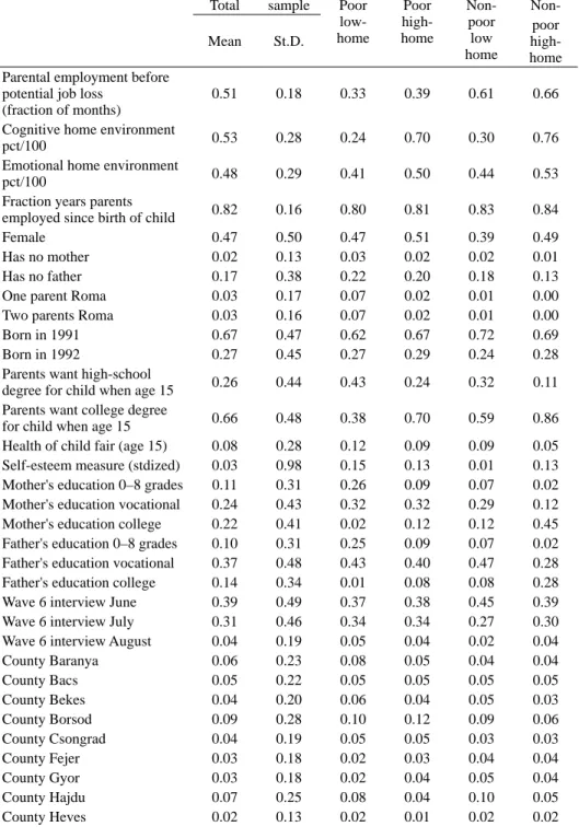
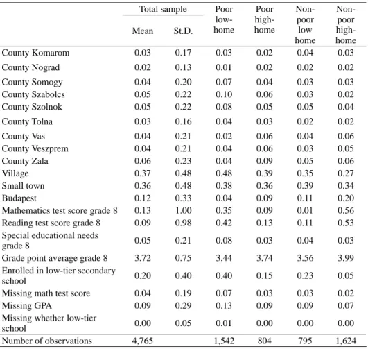
version of the Rosenberg scale), education of the parents, county of residence and whether residence is in a village, small town, larger city or Budapest (the capital city of Hungary), and month of the interview in the sixth wave. The second set of covariates covers educational outcomes prior to the treatment: standardized test scores in reading and mathematics in grade 8, whether the respondent was classified as a student with special educational needs in grade 8, whether the respondent was enrolled in a low-tier (vocational) secondary school in grade 9 and their GPA at the end of grade 8. Summary statistics of these variables in the entire sample and the four subsamples are shown in Table A4 of the Appendix.

3. RESULTS

We want to uncover the effect of a decline in parents’ employment on the probability of adolescents’ completion of secondary school. We compare the completion rate of adolescents whose parents experienced a large decrease in their employment, and whose parents experienced a small decline in employment, separately, to the completion rate of adolescents whose parents did not experience a decrease in their employment. We use the observational data without claiming exogenous variation in parental job loss. The source of parental job loss is not known in our data, preventing us from looking at plant closures or other, arguably exogenous changes. Instead, we condition on a large set of covariates to address the selection of parents into job loss, making use of the rich information in the data. We then provide evidence that conditioning on the covariates controls for the selection.

This identification strategy and the supporting evidence follow the analysis of Stevens – Schaller (2011) and Coelli (2011).

3.1. Main results

We estimate the causal effect in a linear probability model with the binary school completion variable as the dependent variable and the two indicators of large and small decline in parental employment as the main explanatory variables (with no decline being the reference category). One may think of this as a difference- in-differences regression. The main explanatory variables are explicit indicators of differences. The dependent variable is the indicator of successful completion of secondary school, the pre-treatment value of which is zero by definition (no- body completes secondary school before grade 10). We include the pre-recession employment to control for mean reversion, as well as all control variables in the regression.

(10)

The coefficients of main interest are on the indicator variables of both large and small declines in parental employment. To interpret the magnitudes, recall that the fraction of months employed decreased by 40 per cent among those who experienced a large decline, and by 10 per cent among those who experienced a small decline.

Whether our estimates show causal effects is a main issue in our analysis.

Reverse causality is unlikely to be a concern as our measure of the change in parental employment precedes our measure of potential dropping out of secondary school. However, the selection into declining parental employment may create severe omitted variables bias. Parents with unstable job prospects may be over- represented among those who experience a job loss. Families with such parents are likely to be different from other families in many ways that may be related to their children’s dropout probability even without an actual job loss. Arguably, they transmit skills and attitudes and provide environments that decrease the chances of their children’s success in school and beyond. A failure to control for these differences would lead to an estimate of the effect of a parental job loss that is stronger than the true effect. We argue that the exceptionally rich set of control variables capture the entire selection, and we present corroborating evidence in the next section.

In the total sample, adolescents whose parents experienced a large decline in employment were four percentage points less likely to complete secondary school than students whose parents did not experience a decline in their employment (Table 3). The magnitude is substantial: the four per cent difference is more than half of the seven per cent probability of not completing secondary school without a decline in parental employment (corresponding to the 93 per cent baseline completion rate). The difference is half as large, two percentage points, and statistically not significant, for adolescents whose parents experienced a small employment decline. These differences are conditional on all covariates in the regression. We show evidence below that supports the causal interpretation of the estimates.

These estimated average effects conceal substantial heterogeneity. The effect of parental job loss is small and statistically not significant for the adolescents in families with above-median home environment score. That is true for poor families (effect estimate –0.03) and, especially, non-poor families (effect estimate 0.01).

At the same time, the effect is very strong for the adolescents in non-poor families in a less cognitively stimulating home environment. The adolescents in this group with parents who experienced a large employment decline were nine percentage points less likely to complete secondary school than the students whose parents did not experience a decline in their employment with the same income,

(11)

home environment and other covariates. This magnitude is large, and is to be compared to a 93 per cent baseline completion rate in this group (an eight per cent dropout rate). The difference is smaller, i.e. five percentage points and statistically significant on the 10 per cent level in poor families with low-home scores.

The estimated average size of the effect is more than 50 per cent relative to the baseline dropout rate, which is somewhat larger than the effects established in the literature. Using data from the US, Kalil – Wightman (2011) estimated that a parental job loss in childhood leads to a 10 percentage point decrease in the probability of college attendance by age 21, compared to a 50 per cent baseline that corresponds to an effect of 20 per cent. Stevens – Schaller (2011) found that a parental job loss leads to a 1 percentage point increase in the grade retention rate in the subsequent few years that corresponds to a 15 per cent effect. The difference

Table 3. Parental job loss and completion of secondary school Dependent variable:

completed secondary school

Total sample

Poor low-home

Poor high-home

Non-poor low-home

Non-poor high-home Large decline in

parental employment

–0.044** –0.046⁺ –0.032 –0.094* 0.006

(0.013) (0.027) (0.021) (0.037) (0.013)

Small decline in parental employment

–0.023 –0.023 –0.024 –0.022 –0.018

(0.017) (0.031) (0.024) (0.043) (0.028)

Other covariates YES YES YES YES YES

Observations 4,765 1,542 804 795 1,624

Baseline completion

probability 0.93 0.83 0.96 0.93 0.98

Notes: Linear probability model estimates, weighted by sampling weights. Robust standard errors in parenthe- ses. ⁺ p < 0.10, * p < 0.05, ** p < 0.01. Dependent variable: completed secondary school by wave 6 (median age 21). Explanatory variables: large decline in parental employment and small decline in parental employment.

Binary variables indicating whether the fraction of months employed by mother and father (averaged) decreased by at least 25 per cent or 1 to 25 per cent from the pre-recession period (Sept. 2006 to Aug. 2008) to the mid- recession period (Sept. 2008 to Aug. 2010). Pre-recession employment of the parents (the fraction of months employed between Sept. 2006 and Aug. 2008). Cognitively stimulating home environment score and emotion- ally supportive home environment score, the cognitive and emotional subscales of the HOME-SV inventory.

Parental employment between birth of child and 2006 (fraction of months in employment). Other covariates:

Respondent is female; no mother; no father; one parent Roma; two parents Roma; year of birth 1991 or 1992 (reference: 1990 or earlier); aspired to achieve high school education (in 2006); aspired to achieve college education (in 2006); health fair or poor (in 2006); Rosenberg self-esteem score in 2006 (standardized); mother’s education 0–8 grades, vocational school, college (reference: high school); father’s education 0–8 grades, vocational school, college (reference: high school); month of interview (June, July, August, reference May); county of residence; whether residence is in village, small town, large city or Budapest; standardized mathematics and reading test score in grade 8 (2006) and binary indicators for missing values; whether student had special educational needs in grade 8 (2006) and binary indicator for missing values; GPA in grade 8 (2006) and binary indicators for missing values; whether enrolled in low-tier (vocational) secondary school in grade 9 and binary indicator for missing values. Poor vs. non-poor households: below vs. above the permanent income measure median. Low vs. high-home households: below vs. above the cognitively stimulating home environment score median. Baseline completion probability: fraction completed secondary school by wave 6 (median age 21) among respondents whose parents did not experience a decline in employment.

(12)

from what is found in the literature may be due to the fact that the households in Hungary are of an inferior home environment, on average, than the households in the US.

Taken as causal estimates, these results suggest that parental job loss increases the propensity for dropping out of secondary school only in families that do not provide a cognitively stimulating home environment for their children. One interpretation of this finding is that a cognitively stimulating home environment provides a protective factor against dropping out of secondary school during the times of economic distress. Another interpretation is that families that provide such an environment put a high priority on their children’s academic success even during the times of economic distress.

We can only speculate why the effect is greater in non-poor families. Possibly, the effect on secondary school completion is strongest for families whose children are considered enrolling in higher education because the effect of parental job loss has a large effect on its affordability. Having realized that higher education is not an option, children in such families may be more likely to change their behavior and, eventually, drop out of secondary school compared to the children for whom higher education was never an option. Children with plans for higher education are more likely to live in non-poor families, hence we observe the stronger effect on them. Alternatively, it may be due to the stronger stigmatiz- ing effect of job loss among more affluent families, as hypothesized by Brand – Thomas (2014), who found stronger effects in families where parents were particularly unlikely to lose their jobs.

3.2. Results supporting causal interpretation

Selection of families into parental job loss is obviously not random. The recession in 2009 led to more job losses among Hungarian families with a lower propensity to experience such events than in normal times. Nevertheless, one cannot rule out the selection that is correlated with child outcomes. Our strategy of identifying causal effects rests on the assumption that the rich set of covariates controls for selection.

To evaluate whether the covariates adequately control for selection, we estimated regressions with pre-treatment educational outcomes as dependent variables. These outcomes could not have been affected by the subsequent changes in the parents’ employment but may be related to the selection. If our covariates control for nonrandom selection, the coefficients should be zero on both indicators measuring large and small decline in the parental employment. If, however, our covariates do not control for selection in an adequate way, these regressions

(13)

should show significant associations, and the associations should be stronger for large employment decline. The pre-treatment outcomes are the following: whether the student completed the first two years of secondary school, standardized test scores in reading and mathematics in grade 8, GPA in grade 8, whether the student has special educational needs in grade 8, and whether the student is enrolled in a low-tier (vocational) secondary school in grade 9 (as opposed to a higher-tier professional or academic high school).

Table 4 shows the main results related to whether the student completed the first two years of secondary school. In effect, this outcome captures early dropouts.

Note that early dropouts are not in the main sample of our analysis; therefore, the number of observations is higher in Table 4. The results of the other pre-treatment regressions are in Tables from A5 to A9 in the Appendix. The regressions and the structure of the tables are analogous to those reported in Table 3 except the covariates do not include the pre-treatment variable if it is the dependent variable of the placebo regression.

Table 4. Parental job loss and whether student completed the first two years of secondary school, a pre-treatment outcome

Dependent variable:

completed two years of secondary school

Total sample

Poor low-home

Poor high-home

Non-poor low-home

Non-poor high-home

Large decline in parental employment

–0.002 –0.004 –0.001 0.005 0.001

(0.004) (0.011) (0.008) (0.003) (0.001)

Small decline in parental employment

0.007 0.014 0.001 0.009 –0.001

(0.005) (0.013) (0.006) (0.006) (0.001)

Other covariates YES YES YES YES YES

Observations 4,850 1,614 810 800 1,626

Baseline probability of completed two years

0.99 0.96 1.00 0.99 1.00

Notes: Linear probability model estimates, weighted by sampling weights. Robust standard errors in paren- theses. ⁺ p < 0.10, * p < 0.05, ** p < 0.01. Sample contains adolescents who dropped out of secondary school in the first two years (main analysis sample does not include them). Dependent variable: binary indicator of whether student completed two years of secondary school. Explanatory variables, other covariates and subsample definitions: see notes to Table 3. Baseline probability: fraction enrolled in low-tier secondary school among respondents whose parents did not experience a subsequent decline in employment.

None of the associations between completing the first two years of secondary school and subsequent decline in parental employment are significant at the 5 or even 10 per cent level. The point estimates are also very small and do not show

(14)

the same pattern as in the main results in Table 3. While few students do not complete the first two years of secondary school, many of the covariates have statistically significant predictive power, including permanent income, gender, birth year, family structure, ethnicity, and prior educational aspirations. Therefore, the null results with respect to the subsequent decline in parental employment indicate that selection into declining parental employment is captured by the other covariates.

Similarly, the associations with the other pre-treatment outcomes are not statistically significant except for a very few that are of the “wrong” sign; the point estimates are small, and do not show patterns similar to the main results in Table 3 in general (Tables A5–A9 in the Appendix). For example, the sign of the coefficient estimates in the non-poor low-home group, with the strongest association between parental job loss and dropping out, vary across the dependent variables.

Some of them seem to indicate that the selection into subsequent parental decline is positive (lower likelihood of low-tier enrollment, lower probability of special educational needs in grade 8), others seem to suggest a negative selection (lower GPA in grade 8), and sometimes the direction of selection is different for large and small employment declines (test scores).

Taken together, these results suggest that our main estimates reflect causal effects. The association between parental job loss and completion of secondary school represents the effect of parental job loss. When we control for all conditioning variables, selection is unlikely to be an issue.

3.3. Robustness checks

The main results hold across several robustness checks. First, we estimated the regressions on the sample of adolescents not including those who are still in the secondary school. The results in Table A10 (Appendix) are very similar to those in Table 3 with somewhat smaller effects of a small employment decline.

Second, we re-estimated the regression as a logit (results in Table A11 in the Appendix). The relative magnitudes of the coefficient estimates and their statisti- cal significance are the same as in the linear regression presented in Table 3.

Third, we estimated six versions of the regressions in poor versus non-poor groups, defined by one of the six components of the permanent income measure groups instead of the composite measure itself (results in Tables from A12 to A17 in the Appendix). The results for each component are qualitatively similar to the main results. When income or expenditure is used the results are also quantita- tively very similar to the main results. When the value and size of the home, or the history of economic hardship are used, the magnitudes of the effects become

(15)

smaller. For the last two measures the point estimates are as strong in the poor and low-home environment group as in the non-poor and low-home environment group.

Fourth, we estimated three versions of the regressions replacing the composite measure of cognitively stimulating home environment by a sub-measure that contains similar items as the variable used to create the subsamples (results in Tables from A18 to A20 in the Appendix). The first of the three sub-measures contains the items that are closest to measuring permanent income (whether the apartment is light, whether the neighborhood is safe). The second contains items that measure parental investments in the human capital of children (number of books belong- ing to the adolescent child, whether they participate in extra-curricular activities, visited a museum, attended a concert or theater with the family, whether the family has a musical instrument, and whether it subscribes to a newspaper). The third measure contains items related to behavior (whether the adolescent child reads for fun, whether they are encouraged to have a hobby, whether the family talks about what they see on TV, and whether the family is neat and clean).

The results are strongest for the parental investment component. These results replicate our main results. The results with groups using the other two measures (related to permanent income and family behavior) are qualitatively similar, but usually weaker, noisier and statistically insignificant. These results are consistent with our interpretation of the main results. Parental job loss leads to dropping out of secondary school mostly in families with a relatively low priority assigned to human capital investment in their children. Adolescents in families with the same income that invest more in the human capital of their children seem to be substantially more protected from the negative consequences of parental job loss.

We investigated the effect a decline in the mother’s employment separately from the father’s employment decline (results in Table A21 in the Appendix). Our results suggest that the employment decline of the father is as important as the employment decline of the mother. Both show the same pattern (largest effects in non-poor low-home families), and the difference between the two is small and not statistically significant. A large decline in the employment of the mother decreases the probability of completing secondary school by 2.9 percentage points in our sample, while a large decline in the employment of the father leads to a 2.8 percentage point decline. Only the former is significant at the 5 per cent level, but the confidence intervals overlap to a large extent. For the adolescents from non-poor families with a low quality home environment, a large decline in their father’s employment decreases their completion rate by 7 percentage points, compared to a 5 percentage point effect for a large decline in their mother’s employment (the former is significant at the 10 per cent level, and the latter is not). Taken together, the robustness checks strengthen the conclusion of our main analysis.

(16)

4. DISCUSSION AND CONCLUSION

We have documented that a decline in parental employment during secondary school years leads to a substantial increase in dropping out of secondary school even in a country with state-financed (free) secondary education. However, we have shown that this effect depends on the home environment provided by the families prior to the potential job loss of the parents, especially among non-poor families. Parental job loss does not affect the dropout probability of children in the families that have a history of providing a cognitively stimulating home environment for their children. In contrast, it has a strong effect in the families with a history of providing a less stimulating home environment, and the effect is the strongest in the non-poor families.

Certain limitations of our paper should be mentioned. We could not examine some of the potential mechanisms via parental job loss that could affect children’s education: mental stress in the family, family conflict, divorce, erratic and disengaged behavior towards children. On the one hand, we concentrate on stable families to get robust information on the change in employment of the parents.

Therefore, we could not analyze the impacts, e.g. on divorces. On the other hand, other potential mechanisms are not adequately measured in our data. We also note that we analyzed the effect of parental job loss on the probability that their child completes secondary school by age 21. We could not rule out that some of the dropouts will finish their secondary education later.

Nevertheless, our study informs the growing literature on the effect of recessions on student outcomes (Kalil 2013; Brand 2015; Ananat et al. 2017). While recessions may reduce the opportunity costs of staying in school, thus reducing the dropout rate (Betts – McFarland 1995; Long 2015; Adamopoulou – Tanzi 2017), they also increase financial distress for families that experience a job loss, thereby potentially leading to negative effects on investment in the education of their children, thus increasing the dropout rate. Our results highlight the potential heterogeneity of these effects. Children in families that provided a favorable home environment experienced a substantially weaker negative effect. As the home environment is imperfectly correlated with income, even with permanent income, our results may help explain and reconcile some of the conflicting evidence in the literature.

From a broader perspective, our results are also relevant for the long-term consequences of parental investment in the human capital of children throughout the entire childhood (Becker – Tomes 1986; Yeung et al. 2002; Carneiro – Heckman 2003; Todd – Wolpin 2007). The moderating effect of home environment is consistent with the fact that parental investments may have a decisive impact if they are consistently high throughout the childhood. Our results strengthen the case

(17)

for helping families create home environments that enhance the cognitive development of children; such environments appear to be important buffers against the negative shocks from parental job loss.

REFERENCES

Adamecz-Völgyi, A. (2018): Increased Compulsory School Leaving Age Affects Secondary School Track Choice and Increases Dropout Rates in Vocational Training Schools. Budapest Working Papers on the Labour Market, No. BWP – 2018/1. Budapest: Institute of Economics, Centre for Economic and Regional Studies, Hungarian Academy of Sciences.

Adamopoulou, E. – Tanzi, G. M. (2017): Academic Drop-Out and the Great Recession. Journal of Human Capital, 11(1): 35–71.

Ananat, E. O. – Gassman-Pines, A. – Francis, D. V. – Gibson-Davis, C. M. (2017): Linking Job Loss, Inequality, Mental Health, and Education. Science, 356(6343): 1127–1128.

Becker, G. S. – Tomes, N. (1986): Human Capital and the Rise and Fall of Families. Journal of Labor Economics, 4(3): S1–S39.

Betts, J. R. – McFarland, L. L. (1995): Safe Port in a Storm: The Impact of Labor Market Condi- tions on Community College Enrollments. The Journal of Human Resources, 30(4): 741–765.

Bradley, R. H. – Corwyn, R. F. – Caldwell, B. M. – Whiteside-Mansell, L. – Wasserman, G. A.

– Mink, I. T. (2000): Measuring the Home Environments of Children in Early Adolescence.

Journal of Research on Adolescence, 10(3): 247–288.

Brand, J. E. (2015): The Far-Reaching Impact of Job Loss and Unemployment. Annual Review of Sociology, 41(1): 359–375.

Brand, J. E. – Thomas, J. (2014): Job Displacement among Single Mothers: Effects on Children’s Outcomes in Young Adulthood. American Journal of Sociology, 119(4): 955–1001.

Carneiro, P. – Heckman, J. J. (2003): Human Capital Policy. In: Heckman, J. J. – Krueger, A. B.

– Friedman, B. M. (eds): Inequality in America: What Role for Human Capital Policies? Cam- bridge: MIT Press, pp. 77–239.

Charles, K. K. – Melvin, S. Jr. (2004): Job Displacement, Disability, and Divorce. Journal of Labor Economics, 22(2): 489–522.

Coelli, M. B. (2011): Parental Job Loss and the Education Enrollment of Youth. Labour Economics, 18(1): 25–35.

Conger, R. D. – Elder, G. H. (1994): Families in Troubled Times: Adapting to Change in Rural America. New York: Aldine de Gruyter.

Davis-Kean, P. E. (2005): The Infl uence of Parent Education and Family Income on Child Achieve- ment: The Indirect Role of Parental Expectations and the Home Environment. Journal of Family Psychology, 19(2): 294–304.

Flanagan, C. A. – Eccles, J. S. (1993): Changes in Parents’ Work Status and Adolescents’ Adjust- ment at School. Child Development, 64(1): 246–257.

Goldin, C. (1999): Egalitarianism and the Returns to Education during the Great Transformation of American Education. Journal of Political Economy, 107(S6): 65–94.

Gregg, P. – Macmillan, L. – Nasim, B. (2012): The Impact of Fathers’ Job Loss during the Reces- sion of the 1980s on their Children’s Educational Attainment and Labour Market Outcomes.

Fiscal Studies, 33(2): 237–264.

Hilger, N. G. (2016): Parental Job Loss and Children’s Long-Term Outcomes: Evidence from 7 Million Fathers’ Layoffs. American Economic Journal: Applied Economics, 8(3): 247–283.

(18)

Johnson, R. C. – Kalil, A. – Dunifon, R. E. (2012): Employment Patterns of Less-Skilled Workers:

Links to Children’s Behavior and Academic Progress. Demography, 49(2): 747–772.

Kalil, A. (2013): Effects of the Great Recession on Child Development. The ANNALS of the Ameri- can Academy of Political and Social Science, 650(1): 232–250.

Kalil, A. (2015): Inequality Begins at Home: The Role of Parenting in the Diverging Destinies of Rich and Poor Children. In: Amato, P. R. – Booth, A. – McHale, S. M. – Van Hook, J. (eds):

Families in an Era of Increasing Inequality. Springer, pp. 63–82.

Kalil, A. – Wightman, P. (2011): Parental Job Loss and Children’s Educational Attainment in Black and White Middle-Class Families. Social Science Quarterly, 92(1): 57–78.

Kalil, A. – Ziol-Guest, K. M. (2005): Single Mothers’ Employment Dynamics and Adolescent Well- Being. Child Development, 76(1): 196–211.

Kalil, A. – Ziol-Guest, K. M. (2008): Parental Employment Circumstances and Children’s Aca- demic Progress. Social Science Research, 37(2): 500–515.

Kertesi, G. – Kézdi, G. (2007): Children of the Post-Communist Transition: Age at the Time of the Parents’ Job Loss and Dropping Out of Secondary School. The B.E. Journal of Economic Analysis & Policy, 7(2): 1–25.

Linver, M. R. – Brooks-Gunn, J. – Kohen, D. E. (2002): Family Processes as Pathways from In- come to Young Children’s Development. Developmental Psychology, 38(5): 719–734.

Long, B. T. (2015): The Financial Crisis and College Enrollment: How Have Students and Their Families Responded? In: Brown, J. R. – Hoxby, C. M. (eds): How the Financial Crisis and Great Recession Affected Higher Education. Chicago and London: University of Chicago Press, pp. 209–233.

McLoyd, V. C. (1990): The Impact of Economic Hardship on Black Families and Children: Psy- chological Distress, Parenting, and Socioemotional Development. Child Development, 61(2):

311–346.

Rege, M. – Telle, K. – Votruba, M. (2011): Parental Job Loss and Children’s School Performance.

Review of Economic Studies, 78(4): 1462–1489.

Stevens, A. H. – Schaller, J. (2011): Short-Run Effects of Parental Job Loss on Children’s Academic Achievement. Economics of Education Review, 30(2): 289–299.

Todd, P. E. – Wolpin, K. I. (2007): The Production of Cognitive Achievement in Children: Home, School, and Racial Test Score Gaps. Journal of Human Capital, 1(1): 91–136.

Yeung, W. J. – Linver, M. R. – Brooks-Gunn, J. (2002): How Money Matters for Young Children’s Development: Parental Investment and Family Processes. Child Development, 73(6): 1861–

1879.

(19)

APPENDIX

Table A1. The sampling frame, the baseline sample and the analysis sample.

Cohort: 8^th grade students in May 2006

Dataset N

Mean income in

town^a

Mean reading test

score^b

Frac- tion low educated mother^c

Mean # employed parents in family^d

Total student population 119,363 652 – – –

NABC reading test data 109,906 650 –0.08 – –

NABC background

survey 92,588 650 –0.08 0.18 1.5

Agreed to participate

in HLCS 37,027 607 –0.14 0.24 1.4

Baseline HLCS sample^e 10,022 630 –0.11 0.23 1.4

Wave 6. participants^e 6,974 621 –0.07 0.22 1.4

Non-missing

parental employment^e 5,648 619

–0.02 0.19 1.5

Unchanged family^e 4,997 630 0.07 0.11 1.5

Non-missing HOME score ^e 4,850 632 0.07 0.11 1.5

Not early dropout^e 4,765 635 0.09 0.11 1.5

Notes: NABC: National Assessment of Basic Competences; administrative data (http://edecon.mtakti.

hu/?q=node/15).

HLCS: Hungarian Life Course Survey (http://edecon.mtakti.hu/?q=node/16).

a Income per capita in ‘000 HUF in 2006 (1 HUF was approximately 200 USD in 2006). Total income from per- sonal income tax records, divided by total population, in the city/town/village of residence if reported residence in NABC family background survey; city/town/village of school otherwise. Source: TSTAR aggregate statistics (http://adatbank.krtk.mta.hu/adatbazisok___tstar) merged to NABC administrative data.

b Standardized to have zero mean and unit standard deviation in the population of non-special education students. In 2006 special education 8^th-grade students took an adapted version of the reading test so they can receive a background information questionnaire and can be included in the sampling frame of the HLCS. Their test results are included in the overall mean, leading to a negative mean in the population. Source: NABC.

c 0 to 8 grades of education. Source: NABC family background questionnaire.

d Between 0 (no employed parents) and 2 (two employed parents). Source: NABC family background questionnaire.

e Weighted by sampling weights.

(20)

Table A2. Items of the permanent income measure (percentile rankings). Mean values Total

sample

low-home high-home low-home high-home Per capita (equivalent)

family income in 2006 52 28 36 64 73

Per capita (equivalent)

family expenditures in 2005 52 29 37 65 73

Per capita (equivalent)

family expenditures in 2006 52 32 35 65 70

Value of home in 2007 54 30 43 64 73

Size of home (per capita)

in 2007 52 38 40 64 64

How rarely the family experienced economic hardship (when child was age 0–15)

44 39 42 48 48

Mean of items 51 33 39 62 66

Table A3. Items of the cognitive HOME index. Mean values Total

sample

low-home high-home low-home high-home

Child has 20 books or more 0.75 0.47 0.89 0.65 0.94

Musical instrument at home

child can use 0.33 0.11 0.46 0.13 0.52

Family gets a newspaper 0.37 0.21 0.50 0.23 0.48

Child reads for enjoyment 0.50 0.26 0.68 0.24 0.68

Child encouraged to have

hobby 0.86 0.69 0.94 0.79 0.97

Child participates in extra-

curricular activities 0.46 0.24 0.58 0.26 0.66

Child taken to museum last

year 0.49 0.16 0.64 0.22 0.78

Child taken to musical or

drama performance last year 0.48 0.15 0.66 0.15 0.77

When watching TV, parent

discusses program with child 0.73 0.60 0.84 0.56 0.86

Home is not dark 0.90 0.72 0.97 0.92 0.99

Home is reasonably clean 0.93 0.82 1.00 0.93 0.99

Home is minimally cluttered 0.92 0.80 0.98 0.93 0.99

Neighborhood is safe 0.96 0.92 0.99 0.96 0.99

Mean of items 0.67 0.47 0.78 0.54 0.82

Average percentile ranking 53 24 70 30 76

(21)

Table A4. Summary statistics of the control variables Total sample Poor

low- home

Poor high- home

Non- poor low home

Non-

Mean St.D.

poor high- home Parental employment before

potential job loss (fraction of months)

0.51 0.18 0.33 0.39 0.61 0.66

Cognitive home environment

pct/100 0.53 0.28 0.24 0.70 0.30 0.76

Emotional home environment

pct/100 0.48 0.29 0.41 0.50 0.44 0.53

Fraction years parents

employed since birth of child 0.82 0.16 0.80 0.81 0.83 0.84

Female 0.47 0.50 0.47 0.51 0.39 0.49

Has no mother 0.02 0.13 0.03 0.02 0.02 0.01

Has no father 0.17 0.38 0.22 0.20 0.18 0.13

One parent Roma 0.03 0.17 0.07 0.02 0.01 0.00

Two parents Roma 0.03 0.16 0.07 0.02 0.01 0.00

Born in 1991 0.67 0.47 0.62 0.67 0.72 0.69

Born in 1992 0.27 0.45 0.27 0.29 0.24 0.28

Parents want high-school

degree for child when age 15 0.26 0.44 0.43 0.24 0.32 0.11 Parents want college degree

for child when age 15 0.66 0.48 0.38 0.70 0.59 0.86

Health of child fair (age 15) 0.08 0.28 0.12 0.09 0.09 0.05 Self-esteem measure (stdized) 0.03 0.98 0.15 0.13 0.01 0.13 Mother's education 0–8 grades 0.11 0.31 0.26 0.09 0.07 0.02 Mother's education vocational 0.24 0.43 0.32 0.32 0.29 0.12