A characterization of linearized polynomials with maximum kernel

(1)

A characterization of linearized polynomials with maximum kernel

Bence Csajb´ ok, Giuseppe Marino, Olga Polverino, Ferdinando Zullo

^∗

Abstract

We provide sufficient and necessary conditions for the coefficients of a q-polynomial f over Fqⁿ which ensure that the number of dis- tinct roots of f in Fqⁿ equals the degree of f. We say that these polynomials have maximum kernel. As an application we study in detail q-polynomials of degree qⁿ⁻² over Fqⁿ which have maximum kernel and for n≤6 we list all q-polynomials with maximum kernel.

We also obtain information on the splitting field of an arbitrary q- polynomial. Analogous results are proved for q^s-polynomials as well, where gcd(s, n) = 1.

AMS subject classification: 11T06, 15A04

Keywords: Linearized polynomials, linear transformations, semilinear transformations

1 Introduction

A q-polynomial over Fqⁿ is a polynomial of the form f(x) = P

ia_ix^qⁱ, where ai ∈F^qⁿ. We will denote the set of these polynomials byLn,q. Let Kdenote

∗The research was supported by Ministry for Education, University and Research of Italy MIUR (Project PRIN 2012 ”Geometrie di Galois e strutture di incidenza”) and by the Italian National Group for Algebraic and Geometric Structures and their Applica- tions (GNSAGA - INdAM). The first author was supported by the J´anos Bolyai Research Scholarship of the Hungarian Academy of Sciences and by OTKA Grant No. K 124950.

(2)

the algebraic closure of Fqⁿ. Then for every Fqⁿ ≤ L≤ K, f defines an Fq- linear transformation of L, when Lis viewed as an Fq-vector space. IfLis a finite field of sizeq^mthen the polynomials ofLn,qconsidered modulo (x^q^m−x) form an Fq-subalgebra of the Fq-linear transformations of L. Once this field L is fixed, we can define the kernel of f as the kernel of the corresponding F^q-linear transformation ofL, which is the same as the set of roots off inL; and the rank of f as the rank of the corresponding Fq-linear transformation of L. Note that the kernel and the rank of f depend on this field L and from now on we will consider the case L =F^qⁿ. In this case Ln,q considered modulo (x^qⁿ−x) is isomorphic to theFq-algebra ofFq-linear transformations of the n-dimensionalFq-vector spaceFqⁿ. The elements of this factor algebra are represented by ˜L_n,q :={Pn−1

i=0 a_ix^qⁱ: a_i ∈Fqⁿ}. Forf ∈L˜_n,q if degf =q^k then we call k the q-degree of f. It is clear that in this case the kernel of f has dimension at most k and the rank of f is at least n−k.

LetU =hu₁, u₂, . . . , u_ki_F_q be ak-dimensionalFq-subspace ofFqⁿ. It is well known that, up to a scalar factor, there is a unique q-polynomial of q-degree k, which has kernel U. We can get such a polynomial as the determinant of the matrix







x x^q · · · x^q^k u₁ u^q₁ · · · u^q₁^k

...

uk u^q_k · · · u^q_k^k





 .

The aim of this paper is to study the other direction, i.e. when a given f ∈L˜_n,q with q-degreek has kernel of dimension k. If this happens then we say that f is a q-polynomial withmaximum kernel.

If f(x) ≡ a₀x + a₁x^σ + · · · +a_kx^σ^k (mod x^qⁿ − x), with σ = q^s for some s with gcd(s, n) = 1, then we say that f(x) is a σ-polynomial (or q^s- polynomial) with σ-degree (or q^s-degree) k. Regarding σ-polynomials the following is known.

Result 1.1. [7, Theorem 5] LetL be a cyclic extension of a field F of degree n, and suppose that σ generates the Galois group of L over F. Let k be an integer satisfying 1 ≤ k ≤ n, and let a₀, a₁, . . . , a_k be elements of L, not all them are zero. Then the F-linear transformation defined as

f(x) =a₀x+a₁x^σ +· · ·+a_kx^σ^k has kernel with dimension at most k in L.

(3)

Similarly to thes = 1 case we will say that aσ-polynomial is ofmaximum kernel if the dimension of its kernel equals its σ-degree.

Linearized polynomials have been used to describe families of Fq-linear maximum rank distance codes (MRD-codes), i.e. F^q-subspaces of ˜L_n,q of order q^nk in which each element has kernel of dimension at most k. The first examples of MRD-codes found were the generalized Gabidulin codes [3, 5], that is G_k,s = hx, x^q^s, . . . , x^q^s(k−1)i_F_qn with gcd(s, n) = 1; the fact that G_k,s is an MRD-code can be shown simply by using Result 1.1. It is impor- tant to have explicit conditions on the coefficients of a linearized polynomial characterizing the number of its roots. Further connections with projective polynomials can be found in [8].

Our main result provides sufficient and necessary conditions on the coefficients of a σ-polynomial with maximum kernel.

Theorem 1.2. Consider

f(x) = a₀x+a₁x^σ +· · ·+ak−1x^σ^k−1 −x^σ^k,

with σ=q^s, gcd(s, n) = 1 anda₀, . . . , ak−1 ∈Fqⁿ. Thenf(x)is of maximum kernel if and only if the matrix

A=







0 0 · · · 0 a₀ 1 0 · · · 0 a₁ 0 1 · · · 0 a₂ ... ... ... ... 0 0 · · · 1 ak−1







(1)

satisfies

AA^σ· · ·A^σⁿ⁻¹ =I_k,

where A^σⁱ is the matrix obtained from A by applying to each of its entries the automorphism x7→x^σⁱ and I_k is the identity matrix of order k.

An immediate consequence of this result gives information on the splitting field of an arbitrary σ-polynomial, cf. Theorem 4.1.

In Section 3.1 we study in details the σ-polynomials of σ-degree n−2 for each n. For n ≤ 6 we also provide a list of all σ-polynomials with maximum kernel cf. Sections 3.2, 3.3 and 3.4. These results might yield further classification results and examples of Fq-linear MRD-codes.

(4)

2 Preliminary Results

In this section we recall some results of Dempwolff, Fisher and Herman from [4], adapting them to our needs in order to make this paper self-contained.

Let V be a k-dimensional vector space over the field F and let T be a semilinear transformation of V. A T-cyclic subspace of V is an F-subspace of V spanned by{v, T(v), . . .}overFfor somev∈V, which will be denoted by [v]. We first recall the following lemma.

Lemma 2.1. [4, Theorem 1] Let V be an n-dimensional vector space over the field F, σ an automorphism of F and T an invertibleσ-semilinear transformation on V. Then

V = [u₁]⊕. . .⊕[u_r]

for T-cyclic subspaces satisfying dim[u₁]≥dim[u₂]≥. . .≥dim[u_r]≥1.

Theorem 2.2. Let T be an invertible semilinear transformation of V = V(k, qⁿ) of order n, with companion automorphism σ ∈ Aut(Fqⁿ) such that Fix(σ) = F^q. ThenFix(T)is ak-dimensionalF^q-subspace ofV andhFix(T)i_F_qn = V.

Proof. First assume that the companion automorphism of T is x 7→ x^q and that there exists v∈V such that

V =hv, T(v), . . . , T^k−1(v)i_F_qn.

Following the proof of [4, Main Theorem], consider the ordered basis B_T = (v, T(v), . . . , T^k−1(v)) and letAbe the matrix associated withT with respect to the basis BT, i.e.

A=







0 0 · · · 0 α₀ 1 0 · · · 0 α₁ 0 1 · · · 0 α₂ ... ... ... ... 0 0 · · · 1 αk−1







∈F^k×kqⁿ , (2)

where T^k(v) = Pk

i=1αi−1Tⁱ(v) with α₀, . . . , αk−1 ∈ Fqⁿ and, since T is invertible, we have α0 6= 0. Denote by T the semilinear transformation of F^kqⁿ having Aas the associated matrix with respect to the canonical ordered basis B_C = (e₁, . . . ,e_k) of F^kqⁿ and companion automorphism x 7→ x^q. Note

(5)

that cB_T(Fix(T)) = Fix(T), where cB_T is the coordinatization with respect to the basis B_T. Also, since T has order n, we have

AA^q· · ·A^qⁿ⁻¹ =I_k, (3) whereA^qⁱ, fori∈ {1, . . . , n−1}, is the matrix obtained fromAby applying to each of its entries the automorphism x7→x^qⁱ. A vector z= (z₀, . . . , zk−1)∈ F^kqⁿ is fixed byT if and only if











α₀z_k−1^q =z₀ z^q₀+α₁z_k−1^q =z₁ ...

z^q_k−2 +αk−1z_k−1^q =zk−1

Eliminating z₀, . . . , zk−2, we obatin the equation

α^q₀^k−1z_k−1^q^k +α^q₁^k−2z_k−1^q^k−1 +. . .+αk−1z_k−1^q −zk−1 = 0,

which hasq^kdistinct solutions in the algebraic closureKofFqⁿ by the deriva- tive test. Each solution determines a unique vector of Fix(T) in K^k. Also, the set Fix(T) is an Fq-subspace of K^k and hence dim_F_qFix(T) = k. Let {w₁, . . . ,w_k} be an Fq-basis of Fix(T) and note that since |Fix(T)| = q^k, a vector

k

X

i=1

a_iw_i is fixed by T if and only if a_i ∈ Fq. This implies that w₁, . . . ,w_k are alsoK-independent. ThushFix(T)i_K =K^k and {w₁, . . . ,w_k} is also a K-basis of K^k. Denote by φ the K-linear transformation such that φ(w_i) = e_i and by P the associated matrix with respect to the canonical basis B_C, so P ∈ GL(k,K). The semilinear transformation φ◦T ◦φ⁻¹ has companion automorphism x 7→ x^q, order n and associated matrix with respect to the canonical basis P · A · P^−q, where P^−q is the inverse of P in which the automorphism x 7→ x^q is applied entrywise. Note that φ◦T ◦φ⁻¹(ei) =φ(T(wi)) =φ(wi) =ei, hence

P ·A·P^−q=I_k, (4)

i.e.

P^q =P ·A. (5)

By Equations (3) and (5) and using induction we get P^qⁿ =P ·A·A^q·. . .·A^qⁿ⁻¹ =P,

(6)

i.e. P ∈F^k×kqⁿ . This implies that Fix(T) is anFq-subspace ofF^kqⁿ of dimension k and hence Fix(T) = c⁻¹_B

T(Fix(T)) is a k-dimensional subspace of V(k, qⁿ) with the property that hFix(T)i_F_qn =V.

Consider now the general case, i.e. supposeT as in the statement, that is T is an invertible semilinear map of order n with companion automorphism x7→x^q^s and gcd(s, n) = 1. Since gcd(s, n) = 1 there existl, m∈Nsuch that 1 = sl+mn, and hence gcd(l, n) = 1. Then the semilinear transformation T^l has ordern, companion automorphismx7→x^q and Fix(T) = Fix(T^l). By Lemma 2.1, we may write

V = [u1]⊕. . .⊕[ur],

where [u_i] is a T^l-cyclic subspace of V of dimension m_i ≥ 1, for each i ∈ {1, . . . , r}, and Pr

i=1m_i =k. Then we can restrict T^l to each subspace [u_i] and by applying the previous arguments we get that U_i = Fix(T^l|_[u_i_]) is an Fq-subspace of [u_i] of dimension m_i with the property that hU_ii_F_qn = [u_i].

Thus

Fix(T) = Fix(T^l) = U1 ⊕. . .⊕Ur

is an Fq-subspace of dimension k of V with the property that hFix(T)i_F_qn = V.

The existence of a matrixP ∈GL(k,K), with K the algebraic closure of a finite field of order q, satisfying (4) is also a consequence of the celebrated Lang’s Theorem [9] on connected linear algebraic groups. More precisely, by Lang’s Theorem, since GL(k,K) is a connected linear algebraic group, the map M ∈ GL(k,K) 7→ M⁻¹·M^q ∈ GL(k,K) is onto. In Theorem 2.2 it is proved that, if the semilinear transformation of V(k, qⁿ) having A as associated matrix has order n, thenP ∈GL(k,Fqⁿ).

Remark 2.3. Let T be an invertible semilinear transformation of V = V(k, qⁿ) with companion automorphism x 7→ x^q and let K be the algebraic closure of F^qⁿ. Denote by T the semilinear transformation of K^k associated with T as in the proof of Theorem 2.2. If λ ∈ K, then the set E(λ) := {v ∈ K^k: T(v) = λv} is an Fq-subspace of K^k. By [4, page 293], it follows that E(λ) = λ^q−1¹ Fix(T) and by [4, Main Theorem] E(λ) is a k- dimensional F^q-subspace of K^k. Also, when T has order n and λ^q−1¹ ∈ F^qⁿ, by Theorem 2.2, E(λ) is a k-dimensional Fq-subspace contained in F^kqⁿ such that hE(λ)i_F_qn =F^kqⁿ.

(7)

3 Main Results

Now we are able to prove our main result:

Proof of Theorem 1.2. First suppose dim_F_qkerf = k. Then there exist u₀, u₁, . . . , uk−1 ∈Fqⁿ which form an Fq-basis of kerf.

Put u := (u0, u1, . . . , uk−1) ∈ F^kqⁿ. Since u0, u1, . . . , uk−1 are F^q-linearly independent, by [10, Lemma 3.51], we get that B:= (u,u^q^s, . . . ,u^q^s(k−1)) is an orderedFqⁿ-basis ofF^kqⁿ. Also,u^q^sk =a₀u+a₁u^q^s+· · ·+ak−1u^q^s(k−1). It can be seen that the matrix (1) represents the F^qⁿ-linear part of the F^qⁿ-semilinear map σ: v ∈ F^kqⁿ 7→ v^q^s ∈ F^kqⁿ w.r.t. the basis B. Since gcd(s, n) = 1, σ has order n and hence the assertion follows.

Viceversa, letτ be defined as follows

τ:





 x₀ x1

... x_k−1







∈F^kqⁿ 7→A





 x₀ x1

... x_k−1







q^s

∈F^kqⁿ, (6)

where A is as in (1) with the property AA^q^s· · ·A^q^s(n−1) = I_k. Then τ has order n and, by Theorem 2.2, it fixes a k-dimensional F^q-subspace S of F^kqⁿ

with the property that hSi_F_qn =F^kqⁿ.

LetBS = (s₀, . . . ,sk−1) be an Fq-basis ofS and note that, sincehSi_F_qn = F^kqⁿ,BS is also anF^qⁿ-basis ofF^kqⁿ, then denoting byBC the canonical ordered basis of F^kqⁿ, there exists a unique isomorphism φ ofF^kqⁿ such that φ(s_i) = e_i for eachi∈ {1, . . . , k}. Then σ=φ◦τ◦φ⁻¹, whereσ: v∈F^kqⁿ 7→v^q^s ∈F^kqⁿ. Also,

σⁱ =φ◦τⁱ◦φ⁻¹, (7)

for each i∈ {1, . . . , n−1}. Also, by (6) τ(e₀) =e₁,

τ(e₁) =τ²(e₀) = e₂, ...

τ(ek−1) =τ^k(e₀) = (a₀, . . . , ak−1) =a₀e₀+· · ·+ak−1ek−1. So, we get that

τ^k(e₀) =a₀e₀+a₁τ(e₀) +· · ·+ak−1τ^k−1(e₀),

(8)

and applying φ it follows that

φ(τ^k(e₀)) =a₀φ(e₀) +a₁φ(τ(e₀)) +· · ·+ak−1φ(τ^k−1(e₀)).

By (7) the previous equation becomes

σ^k(φ(e₀)) = a₀φ(e₀) +a₁σ(φ(e₀)) +· · ·+ak−1σ^k−1(φ(e₀)).

Put u=φ(e0), then

u^q^sk =a₀u+a₁u^q^s +· · ·+ak−1u^q^s(k−1). This implies that u₀, u₁, . . . , u_k−1 are elements of kerf, where

u= (u₀, . . . , uk−1). Also, they areFq-independent sinceB= (u, . . . ,u^q^s(k−1)) = (φ(e₀), . . . , φ(ek−1)) is an orderedFqⁿ-basis ofF^kqⁿ. This completes the proof.

As a corollary we get the second part of [6, Theorem 10], see also [12, Lemma 3] for the cases= 1 and [11] for the case whenqis a prime. Indeed, by evaluating the determinants inAA^q^s· · ·A^q^s(n−1) =I_k we obtain the following corollary.¹

Corollary 3.1. If the kernel of a q^s-polynomial f(x) =a₀x+a₁x^q^s +· · ·+ ak−1x^q^s(k−1)−x^q^sk has dimension k, then N(a₀) = (−1)^n(k+1).

Corollary 3.2. Let A be a matrix as in Theorem 1.2. The condition AA^q^s· · ·A^q^s(n−1) =I_k

is satisfied if and only if AA^q^s· · ·A^q^s(n−1) fixes e₀ = (1,0, . . . ,0).

Proof. The only if part is trivial, we prove the if part by induction on 0 ≤ i ≤ k−1. Suppose AA^q^s· · ·A^q^s(n−1)e^T_i = e^T_i for some 0 ≤ i ≤ k−1. Then by taking q^s-th powers of each entry we get A^q^sA^q^2s· · ·Ae^T_i = e^T_i . Since Ae^T_i = e^T_i+1 this yields A^q^sA^q^2s· · ·A^q^s(n−1)e^T_i+1 =e^T_i . Then multiplying both sides by A yieldsAA^q^sA^q^2s· · ·A^q^s(n−1)e^T_i+1 =e^T_i+1.

1Forx∈Fqⁿ and for a subfieldFq^m ofFqⁿ we will denote by N_qn/q^m(x) the norm ofx overFq^m and by Tr_qn/q^m(x) we will denote the trace ofxoverFq^m. Ifnis clear from the context andm= 1 then we will simply write N(x) and Tr(x).

(9)

Consider a q^s-polynomial f(x) = a₀x+a₁x^q^s +· · ·+ak−1x^q^s(k−1) −x^q^sk, the matrix A∈F^k×kqⁿ as in Theorem 1.2 and the semilinear map τ defined in (6).

Note that

e^τ₀ = (0,1,0, . . . ,0) = e1

e^τ₀² = (0,0,1, . . . ,0) = e2

...

e^τ₀^k−1 = (0,0,0, . . . ,1) = e_k−1 e^τ₀^k = (a₀, a₁, a₂, . . . , ak−1)

e^τ₀^k+1 = (a₀a^q_k−1^s , a^q₀^s+a₁a^q_k−1^s , a^q₁^s+a₂a^q_k−1^s , . . . , a^q_k−2^s +a^q_k−1^s⁺¹). (8) Hence, if

e^τ₀ⁱ = (Q_0,i, Q_1,i, . . . , Q_k−1,i)

where Q_j,i can be seen as polynomials in a₀, a₁, . . . , ak−1, for i≥0, then e^τ₀ⁱ⁺¹ = (a₀Q^q_k−1,i^s , Q^q_0,i^s +a₁Q^q_k−1,i^s , . . . , Q^q_k−2,i^s +ak−1Q^q_k−1,i^s ),

i.e. the polynomials Q_j,i for 0 ≤ j ≤ k−1 can be defined by the following recursive relations for 0≤i≤k−1:

Q_j,i =

1 ifj =i, 0 otherwise, and by the following relations for i≥k:

Q_0,i+1 =a₀Q^q_k−1,i^s

Q_j,i+1 =Q^q_j−1,i^s +a_jQ^q_k−1,i^s . (9) Now, we are able to prove the following.

Theorem 3.3. The kernel of a q^s-polynomial f(x) = a₀x+a₁x^q^s +· · ·+ a_k−1x^q^s(k−1)−x^q^sk ∈F^qⁿ[x], where gcd(s, n) = 1, has dimension k if and only if

Q_j,n(a₀, a₁, . . . , ak−1) =

1 if j = 0,

0 otherwise. (10)

(10)

Proof. Relations (9) can be written as follows







Q0,i+1

Q_1,i+1 ... Qk−1,i+1







=







0 0 · · · 0 a₀ 1 0 · · · 0 a₁ 0 1 · · · 0 a₂ ... ... ... ... 0 0 · · · 1 ak−1











 Q^q_0,i^s Q^q_1,i^s ... Q^q_k−1,i^s





 ,

withi∈ {0, . . . , n−1}. Also, (Q_0,0, Q_1,0, . . . , Qk−1,0) = (1,0, . . . ,0) ande^τ₀^t = (Q_0,t, . . . , Qk−1,t) for t ∈ {0, . . . , n}. By Theorem 1.2 and by Corollary 3.2, the kernel of f(x) has dimension k if and only ife₀ = (Q_0,0, Q_1,0, . . . , Q_k−1,0) is fixed by AA^q^s· · ·A^q^s(n−1), so this happens if and only if

e^τ₀ⁿ = (Q_0,n, Q_1,n, . . . , Qk−1,n) = (1,0, . . . ,0).

Theorem 3.3 with k = n−1 and s = 1 gives the following well-known result as a corollary.

Corollary 3.4. [10, Theorem 2.24] The dimension of the kernel of a q- polynomial f(x) ∈ Fqⁿ[x] is n−1 if and only if there exist α, β ∈ F^∗qⁿ such that

f(x) = αTr(βx).

Again from Theorem 3.3 we can deduce the following.

Corollary 3.5. [10, Ex. 2.14] The q^s-polynomial a₀x−x^q^sk ∈ Fqⁿ[x], with gcd(s, n) = 1 and 1 ≤ k ≤ n−1, admits q^k roots if and only if k | n and N_qⁿ_/q^k(a0) = 1.

3.1 When the q

^s

-degree equals n − 2

In this section we investigate q^s-polynomials

f(x) = a₀x+a₁x^q^s +· · ·+an−3x^q^s(n−3)−x^q^s(n−2)

with gcd(s, n) = 1. By Theorem 3.3, dim kerf(x) = n−2 if and only if a₀, a₁, . . . , a_n−3 satisfy the following system of equations

(11)











Q_0,n =a₀(a^q_n−4^2s +a^q_n−3^2s^+q^s) = 1,

Q_1,n =a^q₀^sa^q_n−3^2s +a₁(a^q_n−4^2s +a^q_n−3^2s^+q^s) = 0, Q_2,n =a^q₀^2s+a^q_n−3^2s a^q₁^s +a₂(a^q_n−4^2s +a^q_n−3^2s^+q^s) = 0, Q_3,n =a^q₁^2s+a^q_n−3^2s a^q₂^s +a₃(a^q_n−4^2s +a^q_n−3^2s^+q^s) = 0, ...

Q_n−3,n =a^q_n−5^2s +a^q_n−3^2s a^q_n−4^s +a_n−3(a^q_n−4^2s +a^q_n−3^2s^+q^s) = 0,

(11)

which is equivalent to







a₀(a^q_n−4^2s +a^q_n−3^2s^+q^s) = 1,

a₁ =−a^q₀^s⁺¹a^q_n−3^2s =:g₁(a₀, an−3),

a_j =−a^q_j−2^2s a₀−a^q_n−3^2s a^q_j−1^s a₀ =:g_j(a₀, an−3), for 2≤j ≤n−3.

(12)

So, dim_F_qkerf(x) =n−2 if and only ifa₀ and an−3 satisfy the equations a0(gn−4(a0, an−3)^q^2s +a^q_n−3^2s^+q^s) = 1,

an−3 =gn−3(a₀, an−3), and aj =gj(a0, an−3) forj ∈ {1, . . . , n−4}.

Theorem 3.6. Suppose thatf(x) =a₀x+a₁x^q+· · ·+an−3x^qⁿ⁻³−x^qⁿ⁻² has maximum kernel. Then for t ≥2 with gcd(t−1, n) = 1 the coefficients at−2

and an−t are non-zero and, with s=n−t+ 1,

a_n−2t+1a^q_t−2^2s^+q^s =−a^q_n−t^s⁺¹a^q_2t−3^2s . (13) Also, it holds that

−a_n−t(−a^q_t−2^s a^q_3t−4^2s +a^q_2t−3^2s^+q^s) = a^q_t−2^2s^+q^s⁺¹. (14) In particular, for t≥2 with gcd(t−1, n) = 1 we get

N(an−t) = (−1)ⁿN(at−2) (15) and

N(an−2t+1) = (−1)ⁿN(a2t−3), (16)

where n−2t+ 1 and 2t−3 are considered modulo n.

(12)

Proof. Let t≥2 with gcd(t−1, n) = 1 and consider the polynomial F(x) = f(x^q^t), that is,

F(x) = a₀x^q^t +a₁x^q^t+1+· · ·+an−3x^q^n+t−3 −x^q^n+t−2.

Clearly dim_F_qkerF = dim_F_qkerf = n −2. By renaming the coefficients, F(x) can be written as

F(x) =α₀x+α₁x^q^n−t+1+α₂x^q^2(n−t+1)+· · ·+αn−3x^q(n−t+1)(n−3)

+αn−2x^q(n−t+1)(n−2)

=α₀x+α₁x^q^n−t+1+· · ·+α_n−3x^q^3t−3 +α_n−2x^q^2t−2.

Since F(x) has maximum kernel, by the second equation of (12) we get α₀ 6= 0, αn−2 6= 0 and the following relation

− α1

αn−2

=−

− α0

αn−2

q^s+1

−αn−3

αn−2

q^2s

. (17)

The coefficient α_j of F(x) equals the coefficient a_i of f(x) with i ≡n−t+ j(1−t) (mod n), in particular











α₀ =an−t, α₁ =an−2t+1, α_n−3 =a_2t−3, αn−2 =at−2, αn−4 =a3t−4,

(18)

and by (17), we get that at−2 and an−t are nonzero, and an−2t+1a^q_t−2^2s^+q^s =−a^q_n−t^s⁺¹a^q_2t−3^2s , which gives (13). The first equation of (12) gives

− α₀ αn−2

−αn−4

αn−2

q^2s

+

−αn−3

αn−2

q^2s+q^s!

= 1, that is,

−α0(−α^q_n−2^s α^q_n−4^2s +α^q_n−3^2s^+q^s) = α^q_n−2^2s^+q^s⁺¹. Then (18) and αn−4 =a3t−4 imply

−an−t(−a^q_t−2^s a^q_3t−4^2s +a^q_2t−3^2s^+q^s) = a^q_t−2^2s^+q^s⁺¹,

(13)

which gives (14). By Corollary 3.1 with s=n−t+ 1 we obtain N

− α₀ αn−2

= 1, and taking (18) into account we get

N(an−t) = (−1)ⁿN(at−2).

Then (13) and the previous relation yield

N(an−2t+1) = (−1)ⁿN(a2t−3).

Proposition 3.7. Let f(x) be a q^s-polynomial with q^s-degree n−2 and with maximum kernel. If the coefficient of x^q^s is zero, then n is even and f(x) = αTr_qⁿ_/q²(βx) for someα, β ∈F^∗qⁿ.

Proof. We may assume f(x) =a0x+a1x^q^s+· · ·+an−3x^q^s(n−3)−x^q^s(n−2) with a₁ = 0. By the second equation of (12), it follows thatan−3 = 0. By the third equation of (12), we get thata_j = 0 for every odd integer j ∈ {3, . . . , n−3}.

If j is even then we have

a_j = (−1)²^ja^q₀^sj^+q^s(j−2)^+···+q^2s⁺¹. (19) If n−3 is even, then this gives us a contradiction withj =n−3. It follows thatn−3 is odd and hencenis even. By N(a₀) = (−1)ⁿ, there existsλ ∈F^∗qⁿ

such that a₀ =−λ^1−q^s(n−2). So, by (19) we get a_j =λ^q^js^−q^s(n−2), and hence f(x) = Tr_qⁿ_/q²(λx)

λ^q^s(n−2) .

In the next sections we list all the q^s-polynomials of Fqⁿ with maximum kernel for n ≤ 6. By Corollaries 3.4 and 3.5 the n ≤ 3 case can be easily described hence we will consider only the n∈ {4,5,6} cases.

For f(x) = Pn−1

i=0 a_ix^qⁱ ∈ L˜_n,q we denote by ˆf(x) := Pn−1

i=0 a^q_iⁿ⁻ⁱx^qⁿ⁻ⁱ the adjoint (w.r.t. the symmetric non-degenerate bilinear form defined by hx, yi= Tr(xy)) off.

By [1, Lemma 2.6], see also [2, pages 407–408], the kernel off and ˆf has the same dimension and hence the following result holds.

(14)

Proposition 3.8. If f(x) ∈ L˜_n,q is a q^s-polynomial with maximum kernel, then fˆ(x) is a q^n−s-polynomial with maximum kernel.

This will allow us to consider only thes ≤n/2 case.

3.2 The n = 4 case

In this section we determine the linearized polynomials over Fq⁴ with maximum kernel. Without loss of generality, we can suppose that the leading coefficient of the polynomial is −1.

Because of Proposition 3.8, we can assumes= 1. Corollaries 3.4 and 3.5 cover the cases when the q-degree of f is 1 or 3 so from now on we suppose f(x) =a0x+a1x^q−x^q². If a1 = 0 then we can use again Corollary 3.5 and we get a₀x−x^q², with N_q⁴_/q²(a₀) = 1. Suppose a₁ 6= 0. By Equation (12), we get the conditions

(

a₀(a^q₀² +a^q₁²^+q) = 1, a₁ =−a^q+1₀ a^q₁², which is equivalent to

N_q⁴_/q(a₀) = 1, a^q+1₁ =a^q₀²^+q+1−a^q₀, see (A1) of Section 5.

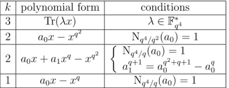
Here we list the q-polynomials of L4,q with maximum kernel, up to a non-zero scalar inF^∗_q⁴. Applying the adjoint operation we can obtain the list of q³-polynomials over Fq⁴ with maximum kernel. In the following table the q-degree will be denoted by k.

k polynomial form conditions

3 Tr(λx) λ∈F^∗_q⁴

2 a₀x−x^q² N_q⁴_/q²(a₀) = 1 2 a₀x+a₁x^q−x^q²

N_q⁴_/q(a₀) = 1 a^q+1₁ =a^q₀²^+q+1−a^q₀ 1 a₀x−x^q N_q⁴_/q(a₀) = 1

Table 1: Linearized polynomials of Fq⁴ with maximum kernel withs = 1

(15)

3.3 The n = 5 case

In this section we determine the linearized polynomials over Fq⁵ with maximum kernel. Without loss of generality, we can suppose that the leading coefficient of the polynomial is −1. Because of Proposition 3.8, we can assume s ∈ {1,2}. Corollaries 3.4 and 3.5 cover the cases when the q^s-degree of f is 1 or 4. First we suppose that f has q^s-degree 3, i.e.

f(x) =a0x+a1x^q^s+a2x^q^2s −x^q^3s.

From (12), f(x) has maximum kernel if and only ifa₀,a₁ and a₂ satisfy the following system:







a₁ =−a^q₀^s⁺¹a^q₂^2s,

−a^q₀^3s^+q^2s⁺¹a^q₂^4s +a^q₂^2s^+q^sa₀ = 1, a₂ =−a^q₀^2s⁺¹+a^q₂^3s^+q^2sa^q₀^2s^+q^s⁺¹, which is equivalent to







N(a₀) = 1, a₁ =−a^q₀^s⁺¹a^q₂^2s,

−a^q₀^3s^+q^2s⁺¹a^q₂^4s +a₀a^q₂^2s^+q^s = 1, see (A2) of Section 5.

Suppose now that the q^s-degree is 2, i.e.

f(x) = a₀x+a₁x^q^s −x^q^2s.

By Theorem 3.3 the polynomial f(x) has maximum kernel if and only if its coefficients satisfy

(

a₀(a^q₀^2sa^q₁^3s+a^q₁^s(a^q₀^3s+a^q₁^3s^+q^2s)) = 1, a^q₀^s⁺¹(a^q₀^3s +a^q₁^3s^+q^2s) +a₁ = 0,

which is equivalent to

N(a₀) =−1,

a^q₀^s +a^q₁^s⁺¹ =a^q₀^2s^+q^s⁺¹a^q₁^3s, see (A3) of Section 5.

Here we list theq^s-polynomials, s∈ {1,2} of L_5,q with maximum kernel, up to a non-zero scalar inF^∗_q⁵. Applying the adjoint operation we can obtain the list of q^t-polynomials, t ∈ {3,4}, over Fq⁵ with maximum kernel. As before, the q^s-degree is denoted by k.

(16)

k polynomial form conditions

4 Tr(λx) λ∈F^∗q⁵

3 a₀x+a₁x^q^s +a₂x^q^2s−x^q^3s







N(a₀) = 1 a₁ =−a^q₀^s⁺¹a^q₂^2s

−a^q₀^3s^+q^2s⁺¹a^q₂^4s +a₀a^q₂^2s^+q^s = 1 2 a₀x+a₁x^q^s −x^q^2s

N(a0) = −1

a^q₁^s⁺¹+a^q₀^s =a^q₁^3sa^q₀^2s^+q^s⁺¹

1 a₀x−x^q^s N(a₀) = 1

Table 2: Linearized polynomials of Fq⁵ with maximum kernel withs∈ {1,2}

3.4 The n = 6 case

In this section we determine the linearized polynomials over Fq⁶ with maximum kernel. Without loss of generality, we can suppose that the leading coefficient of the polynomial is −1. Because of Proposition 3.8, we can assume s = 1. Corollaries 3.4 and 3.5 cover the cases when the q-degree of f is 1 or 5. As before, denote by k the q^s-degree off.

We first consider the case k = 2, i.e. f(x) = a₀x+a₁x^q^s − x^q^2s. By Theorem 3.3, f(x) has maximum kernel if and only if the coefficients satisfy







N(a₀) = 1,

(a^q₀+a^q+1₁ )^q³ =a^q₀⁵^+q⁴^+q³(a^q₀+a^q+1₁ ), a^q₁⁴a^q₀³ +a^q₁²(a^q₀⁴ +a^q₁⁴^+q³) = − ^a¹

a^q+1₀ , see (A4) of Section 5.

Ifk = 3, then f(x) =a₀x+a₁x^q^s +a₂x^q^2s −x^q^3s, and by Theorem 3.3 it has maximum kernel if and only the coefficients fulfill











N(a₀) = 1,

a^q₀³^+q+1+a^q₂³a^q₁²a^q+1₀ −a^q₂a₁ =a^q₀, a^q+1₂ =−a^q₀³^+q²^+q+1a^q₁⁴ −a^q₁, a^q+1₁ =a₂a^q₀+a^q₀²^+q+1a^q₂³,

see (A5) of Section 5. Note that a₁ = 0 if and only if a₂ = 0 and in this case we get the trace over Fq³.

(17)

Finally, let k = 4. Then the polynomial f(x) = a₀x+a₁x^q^s +a₂x^q^2s + a₃x^q^3s −x^q^4s has maximum kernel if and only if the coefficients satisfy











N(a₀) = 1,

a₀(−a^q₀⁴^+q² +a^q₃⁵^+q⁴a^q₀⁴^+q³^+q² +a^q₃²^+q) = 1, a₁ =−a^q+1₀ a^q₃²,

a₂ =−a^q₀²⁺¹+a^q₃³^+q²a^q₀²^+q+1,

a₃ =a^q₃⁴a^q₀³^+q²⁺¹+a^q₃²a^q₀³^+q+1−a^q₀³^+q²^+q+1a^q₃⁴^+q³^+q², see (A6) of Section 5.

Here we list theq-polynomials ofL_6,q with maximum kernel, up to a non- zero scalar in F^∗q⁶. Applying the adjoint operation we can obtain the list of q⁵-polynomials over Fq⁶ with maximum kernel.

(18)

Table3:LinearizedpolynomialsofFq6withmaximumkernelwiths=1 kpolynomialformconditions 5Trq6/q(λx)λ∈F∗ q6 4a0x+a1xq +a2xq2 +a3xq3 −xq4

                

a16=0 N(a0)=1 a0(−aq4+q2 0+aq5+q4 3aq4+q3+q2 0+aq2+q 3)=1 a1=−aq+1 0aq2 3 a2=−aq2+1 0+aq3+q2 3aq2+q+1 0 a3=aq4 3aq3+q2+1 0+aq2 3aq3+q+1 0−aq3+q2+q+1 0aq4+q3+q2 3 4Trq6/q2(λx)λ∈F∗ q6 3a0x+a1xq +a2xq2 −xq3

        

N(a0)=1 aq3+q+1 0+aq3 2aq2 1aq+1 0−aq 2a1=aq 0 aq+1 2=−aq3+q2+q+1 0aq4 1−aq 1 aq+1 1=a2aq 0+aq2+q+1 0aq3 2 3Trq6/q3(λx)λ∈F∗ q6 2a0x+a1xq −xq2

        

a16=0 N(a0)=1 (aq 0+aq+1 1)q3 =aq5+q4+q3 0(aq 0+aq+1 1) aq4 1aq3 0+aq2 1(aq4 0+aq4+q3 1)=−a1 aq+1 0 2a0x−xq2 Nq6/q2(a0)=1 1a0x−xq Nq6/q(a0)=1