Hilbert geometries with Riemannian points

https://doi.org/10.1007/s10231-019-00901-5

Hilbert geometries with Riemannian points

Árpád Kurusa^1,2

Received: 27 November 2018 / Accepted: 28 August 2019 / Published online: 7 September 2019

© The Author(s) 2019

Abstract

If a Hilbert geometry of twice differentiable boundary has two quadratic infinitesimal spheres, then the Hilbert geometry is a Cayley–Klein model of the hyperbolic geometry.

Keywords Hilbert geometry·Projective metric·Beltrami’s theorem·Riemannian point· Geometric tomography·(−1)-Chord function

Mathematics Subject Classification 53A35·52A20

1 Introduction

LetC Ddenote the open segment of the pointsC,D∈Rⁿ(n=1,2, . . .), and if it is on the straight lineA Bof points A,B∈Rⁿ, then let(A,B;C,D)denote thecross-ratioof these points. IfMis an open, strictly convex, and bounded subset ofRⁿ (n=2,3, . . .), then the functiond:M×M→Rdefined by

d(A,B)=

0, ifA=B,

1

2ln(A,B;C,D), ifA=B,whereC D=M∩A B,

is ametric onM[4, p. 297] which satisfies the strict triangle inequality, i.e.,d(A,B)+ d(B,C)=d(A,C)if and only ifB ∈ AC∪ {A,C}. This functiondis called theHilbert metric on_M, and_Mis itsdomain. Such pairs(M,d)are calledHilbert geometries.

Hilbert geometries are Finslerian manifolds [4, (29.6)]. We call a point P of a Hilbert geometry(M,d) Riemannian if the Finsler norm on TPM is quadratic. By Beltrami’s theorem [1,2] (see also [4, (29.3)]), a Hilbert geometry is Riemannian if and only if it is a Cayley–Klein model of the hyperbolic geometry.

In this paper, we prove in Theorem4.4that

Research was supported by NFSR of Hungary (NKFIH) under grant numbers K 116451 and KH_18 129630, and by the Ministry of Human Capacities, Hungary grant 20391-3/2018/FEKUSTRAT.

B

kurusa@math.u-szeged.hu

1 Bolyai Institute, University of Szeged, Aradi vértanúk tere 1, Szeged 6725, Hungary 2 Alfréd Rényi Institute of Mathematics, Hungarian Academy of Sciences, Reáltanoda u. 13-15,

Budapest 1053, Hungary

a Hilbert geometry in the plane hastwoRiemannian points if and only if it is a Cayley–

Klein model of the hyperbolic geometry.

For the proof, we need the assumption that the boundary is twice differentiable at the points, where the line joining the two Riemannian points intersects the boundary. Theorem5.2shows that this assumption is also necessary.

Theorem4.4is also formulated in the language of geometric tomography [7] by Theo- rem5.3:

the twice differentiable boundary of a strictly convex bounded domain in the plane is an ellipse if and only if its(−1)-chord functions are quadratic at two inner points.

2 Notations and preliminaries

Points ofRⁿ are denoted by capital lettersA,B, . . ., vectors are−→

A Bora,b, . . ., but we use these latter notations also for points if the origin is fixed. We denote the interior of the convex hull of a point setPbyP.

ForC ∈A B, theaffine ratio(A,B;C)is defined by(A,B;C)−→

BC=−→

AC, and it satisfies (A,B;C,D)=(A,B;C)/(A,B;D)[4, p. 243].

If a Euclidean metricd_eis given, then the length of a segmentA B, or of a vector−→

A B=x is denoted by|A B| = |x| =d_e(A,B).

We use the usual big-O and little-onotation. To indicate derivatives of a function or a map, we use prime, dot orDappropriately.

If the domainMof the Hilbert geometry(M,d)is inRⁿ, then we identify the tangent spacesTPMwithRⁿby the mapıP:v→ P+v. This way, the Finsler functionF_M:M× Rⁿ →Rassociated with the Hilbert metricdcan be given at a pointP∈Mby

F_M(P,v)= 1 2

1 λ⁻_v + 1

λ⁺_v

, (2.1)

wherev ∈ TPM, and λ^±_v ∈ (0,∞]is such that P_v^± := P ±λ^±_vv ∈ ∂M[4, (50.4)].¹ Equation (2.1) implies thatıPmaps the indicatrix of normF_M(P,·)into the strictly convex setB^M_P ⊂Rⁿ, theinfinitesimal ball, with boundary

S^M_P :=∂B^M_P = {2(P_v⁺−P)(P,P_v⁺;P_v⁻):v∈TPM}, theinfinitesimal sphere. Observe here that

if is a projective transformation on the projective completionPⁿ ofRⁿ, then its derivative˙ is anaffinetransform from each tangent spaceTPMof MontoT ₍P) (M), and (˙ S^M_P )≡S _(P) ^(M)holds.

(2.2) From now on, we work only in the plane unless explicitly said otherwise.

So, infinitesimal spheres are calledinfinitesimal circlesand denoted byC^M_P .

If a Euclidean metric is provided, then we frequently use the notationu_ϕ =(cosϕ,sinϕ).

Further, if a bounded open domainD⊂R²is starlike with respect to a pointP ∈D, then we usuallypolar parameterizetheboundary∂Dwith a functionr: [−π, π)→R²defined byr(ϕ)=r(ϕ)u_ϕ ∈∂D,wherer >0 is theradial functionof_Dwith respect to thebase

1Ifλ^±v = ∞, thenP_v^±is an ideal point.

point P. For any ellipseEwith centerPthere exists uniqueω∈(−π/2, π/2]anda≥b>0 such that

1

r²(ϕ) = cos²(ϕ−ω)

a² +sin²(ϕ−ω)

b² (2.3)

is thepolar equationwith respect to originP.

We also use the notation d := {λd : λ ∈ R} for the line through the origin with nonvanishing directional vectord, andξ =u_ξ as a short hand in the plane.

The following result is a rephrase of [5, Stable Manifold Theorem, p. 114]. See also [6, Theorem 4.1]!

Theorem 2.1 Let_N0⊂R²be a neighborhood of the origin0, and let the mapping:N0→ R²be of class C^l(l∈ [1,∞]).

If there are linearly independent vectorsuandvsuch that(w) = wfor everyw ∈ u∩N0, andD_(0,0)v=kvfor some k∈(0,1), then in some neighborhoodN ⊆N0of0 the set{w∈N :^(r)(w)→0as r → ∞}is the graph of a C^lfunction fromv∩Ntou∩N.

Notice that^(r)refers to ther-th iterate, rather than, e.g., ther-th derivative.

Finally, we need the following easy consequence of [4, (28.11)]:

Letbe an affine line through point P of the Hilbert plane(M,d). Let I and J be the points whereintersects∂M. Let L be the common (maybe ideal) point of the tangents of_Mat I and J . Then the tangents of_C^M_P at its intersections withgo through point L.

(2.4)

3 Utilities

Although it is known that the hyperbolic geometry is a Riemannian manifold, so its infinites- imal spheres are quadratic, the following result gives some more details.

Lemma 3.1 LetEebe the ellipse x²+_e^y2² =1, and let P=(p,0), where p∈(−1,1). Then C^E_P^eis the ellipse ^(x−p)2

a² +_b^y22 =1, where a=1−p²and b=e 1−p². Proof. According to (2.2), we can assume thate=1 without loss of generality.

Let lineP+_ξ intersectEein the pointsP±λ_±u_ξ. Then 1=λ²_±+p²∓2pλ_±cosξ, henceλ±= ±pcosξ+

1−p²sin²ξ. Thus (2.1) gives 1

r²(ξ) = 1 λ+ + 1

λ−

2

= 1−p²sin²ξ

(1−p²)² = cos²ξ

(1−p²)² + sin²ξ 1−p². Notice that_C^E_P^¯eis a circle if and only if 1−p²=e

1−p², i.e.,p= ±√

1−e²which can only happen ife<1. In this case,Pis a focus ofEe.

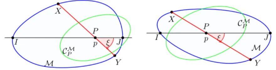
From now on, we always use the following general configuration: Pis a point of a 2- dimensional Hilbert geometry(M,d);is a straight line throughP;IandJ are the points whereintersects∂M;acoordinate system is chosen²such thatI =(−1,0),J =(1,0), andP=(p,0), where−1< p<1;XandY are the points whereP+ξintersects∂M. Figure1shows qualitative depictions of what we have in general.

2Point(0,1)will always be chosen outsideso as to help calculations.

I J M

C_P^M X

Y ξ P

p I MJ

C^M_P X

Y ξ

P p

Fig. 1 Qualitative depiction of infinitesimal circles in Hilbert planes

Observe that forX∈∂Mwe have 2F_M(P,X−P)−1=1/λ⁻_X−P>0 by (2.1), so, as a continuous function takes its minimal value, there is a suitably smallε >0 such that the map

P: Z→P(Z)=P+(P−Z) 1

2F_M(P,Z−P)−1 (3.1) is well defined on the Minkowski sumM^ε:=∂M+εB², whereB²is the unit ball at(0,0).

ChoosetheEuclidean metricd_esuch that{(1,0), (0,1)}is an orthonormal basis, and polar parameterizeC^M_P with respect toPbyr: [−π, π)ξ →r(ξ)u_ξ∈R². Then (2.1) gives

1

|X P|+ 1

|PY| = 2

r(ξ). (3.2)

Thusris twice differentiable if∂Mis twice differentiable, and r(0)=2|I P||P J|

|I J| =1−p², hence 2|I P| −r(0)=(1+p)². (3.3) Lemma 3.2 Let X∈I+εB², and set Y =P(X). Let(x,y)=X−I and(u, v)=J−Y .

Then

v

1+ u

1−p +O(u²)

=y 1−p

1+p +x 1−p

(1+p)² +O(x²)

, (3.4)

and

−u=x(1−p)²

(1+p)² −y 2r(0)

(1+p)³ +x²2(1−p)²

(1+p)⁴ −x yr(0)2(3−p) (1+p)⁵ + +y² 1

(1+p)³

−(1−p)+2(r(0))²

(1+p)³ + r(0) 1+p

+ +O(x³)+O(x²y)+o(y²).

(3.5)

Proof Letu_ξ =(X−P)/|X−P|. Then we clearly have_1+p−x^y = −tanξ = _1−p−u^v , so the expansions of_1−p−u¹ and₁₊¹_p−x give (3.4).

To prove (3.5), we are estimating−ufor the second order ofxandy. We start with (3.2) and use (3.3) as

−u= |PY|cosξ− |P J| = cosξ

r(ξ)2 −_{|X P|}¹ −(1−p)=r(ξ)|X P|cosξ

2|X P| −r(ξ) −(1−p)

=r(ξ)(1+p−x)−(1−p)(2|X P| −r(ξ))

2|X P| −r(ξ) =r(ξ)(2−x)−2(1−p)|X P| 2|X P| −r(ξ)

= (r(ξ)−r(0))(2−x)+r(0)(2−x)−2(1−p)|I P| +2(1−p)(|I P| − |X P|) 2|X P| −r(ξ)

= (r(ξ)−r(0))(2−x)−xr(0)+2(1−p)(|I P| − |X P|) 2|X P| −r(ξ)

shows. Next we estimate|X P|by the binomial series so that

|X P| =((|I P| −x)²+y²)^1/2= |I P| −x+ y²/2

|I P| −x +O(y⁴)

= |I P| −x+y² 2

1

|I P|+O(x)

+O(y⁴)= |I P| −x+ y²/2

1+p+O(x y²)+O(y⁴).

(3.6) Substitution of this into the previous formula and some rearrangements result in

−u= (1−p)

2x−_1+p^y2

+(2−x)(r(ξ)−r(0))−x(1−p²)

2|X P| −r(ξ) +O(x y²)+O(y⁴)

= x(1−p)(1−p²)−(1−p)y²+(2−x)(1+p)(r(ξ)−r(0))

(2|X P| −r(ξ))(1+p) +

+O(x y²)+O(y⁴). (3.7)

To estimate this, we need to considerr(ξ)−r(0)and 1/(2|X P| −r(ξ)). We use the binomial series and (3.6) to get

1

|X P| = 1

|I P| −(|I P| − |X P|) =

1+p−

x− y²/2

1+p +O(y²x)+O(y⁴)₋1

= 1

1+p+ x

(1+p)² − y²/2

(1+p)³ + x²

(1+p)³ +O(x y²)+O(y⁴)+O(x³).

This, as sinξ= −y/|X P|, leads to ξ =sinξ+O(ξ³)= −y

|X P|+O(y³)= −y

1+p− yx

(1+p)² +O(y³)+O(yx²). (3.8) Substitution of this into the Taylor expansion ofrgives

(1+p)(r(ξ)−r(0))

=(1+p)

ξr(0)+ξ²

2r(0)+o(ξ²)

=

−y− yx 1+p

r(0)+ y² 1+p

r(0)

2 +o(y²)+O(yx²)+O(y²x).

(3.9)

Again the binomial series, and then (3.3), (3.6), and (3.9) result in 1

2|X P| −r(ξ) = 1

(2|I P| −r(0))−(2(|I P| − |X P|)+(r(ξ)−r(0)))

=

(1+p)²−(2(|I P| − |X P|)+(r(ξ)−r(0)))₋₁

= 1

(1+p)² +2x−y^r₁₊⁽⁰⁾_p

(1+p)⁴ +O(x²)+O(x y)+O(y²). (3.10)

Putting estimates (3.9), (3.10), and (3.8) into (3.7) and confining ourselves to summands of degree less than three, we obtain

−u+O(x³)+O(x²y)+o(y²)

= 1

(1+p)³ +2x−y^r_1+p⁽⁰⁾ (1+p)⁵

(x(1−p²)−y²)(1−p)+(2−x)(1+p)(r(ξ)−r(0))

= 1

(1+p)³ +2x−y^r_1+p⁽⁰⁾ (1+p)⁵

(x(1−p²)−y²)(1−p)+

+ 1

(1+p)³ +2x−y^r₁₊⁽⁰_p⁾ (1+p)⁵

(2−x)

−y− yx 1+p

r(0)+ y² 1+p

r(0) 2

= (x(1−p²)−y²)(1−p)

(1+p)³ +(2x²(1+p)−x yr(0))(1−p)²

(1+p)⁵ −

−2y−x y

(1+p)³ + 2x y

(1+p)⁴ +4x y−2y^2r₁₊⁽⁰⁾_p (1+p)⁵

r(0)+ y²

(1+p)⁴r(0),

where the summands that are estimated byO(x³)+O(x²y)+o(y²)was left out. Collecting the terms by their powers gives

−u=x(1−p)²

(1+p)² −y 2r(0)

(1+p)³ +x²2(1−p)² (1+p)⁴ −

−x y r(0) (1+p)³

(1−p)²

(1+p)² −1+ 2

1+p + 4

(1+p)² +

+y² 1 (1+p)³

−(1−p)+2(r(0))²

(1+p)³ + r(0) 1+p

+O(x³)+O(x²y)+o(y²).

This implies (3.5) after reordering the summands.

4 Hilbert geometries with two Riemannian points

In what follows, we always assume that P and Q are Riemannian points of the Hilbert plane(M,d), = P Q is the x-axis of the chosen coordinate system, I and J are the intersection points ofand∂M,I = (−1,0),J = (1,0), P = (p,0)andQ = (q,0), where−1<q< p<1. Further,tIandtJare the respective tangents ofMatIandJ, and the tangents ofC^M_Q andC^M_P at their respective intersections witharet^Q_I,t^Q_J andt^P_I,t^P_J, respectively.

Notice that the infinitesimal circleC^M_P is now an ellipse, so it is of form (2.3) in any Euclidean metric. Observe that differentiation of (2.3) yields

r(ϕ)=1 a² − 1

b²

sin(2ϕ−2ω) 2 r³(ϕ), r(ϕ)=1

a² − 1 b²

r²(ϕ)

cos(2ϕ−2ω)r(ϕ)+3 sin(2ϕ−2ω)

2 r(ϕ)

. Further, using

1

r²(0)− 1

r²(π/2) = cos²ω

a² +sin²ω

b² −sin²ω

a² −cos²ω b² =1

a² − 1 b²

cos(2ω),

we obtain

r(0)= −r³(0) 1

r²(0) − 1 r²(π/2)

tan(2ω)

2 ,

r(0)= 1

r²(0)− 1 r²(π/2)

r³(0)+3(r(0))²

r(0) . (4.1)

Lemma 4.1 If∂Mis twice differentiable at I and J , then there is a unique ellipseEtouching Mat I,J such thatC^E_Q≡C^M_Q andC^E_P≡C^M_P .

Proof If t^Q_I intersectst^P_J, thent_I also intersects t_J in a point, say L, by (2.4). Choose a straight linelthrough Lthat avoidsM, and let be a perspectivity that takeslinto the ideal line ofR². Then, by (2.2), (˙ C^M_Q )≡C _(Q) ^(M), and(˙ C^M_P )≡C _(P) ^(M), hold, where the derivative˙ of is anaffinetransform. As affinities keep quadraticity, (Q)and (P) are Riemannian points in the Hilbert geometry( (M),d _(M)), so we can assume without loss of generality thatt^Q_I t^P_J.

Fix the Euclidean metricdin whichC^M_Q is a circle andd(I,J)=2. SinceC^M_Q is a circle, t^Q_I andt^P_J, and, by (2.4), alsotI andtJ are perpendicular to lineQ P. Figure2shows what we have.

Thus we haver(0)=0 and alsor(0) =r³(0) ₁

r²(0)−_r2(π/¹ 2)

by (4.1). So equation (3.5) reduces to

−u=x(1−p)² (1+p)² + x²

r(0)

2(1−p)³ (1+p)³ − y²

r(0)

(1−p)² (1+p)²+ +y²r(0)(1−p)²

(1+p)² 1

r²(0)− 1 r²(π/2)

+O(x³)+O(x²y)+o(y²).

(4.2)

Assume from now on thatX∈∂M, hence alsoY =P(X)∈∂M.

SincetI andtJ are perpendicular to lineQ P, basic differential geometry gives that the respective curvatures of∂MatIandJ are

κI:= lim

x→0

2x

y² and κJ := lim

u→0

2u

v². (4.3)

So, dividing (4.2) by the square of (3.4) leads to

M

I J

Q q

C_Q^M

P p C_P^M

t^Q_I t^P_J

tI tJ

M

I J

Q q C_Q^M

P p C_P^M

t^Q_I t^P_J

tI tJ

Fig. 2 Riemannian pointsQ,Pin a Hilbert planeM

κJ = lim

u→0

2u v² = lim

u→0

−2x y² + 2

r(0)−2r(0) 1

r²(0)− 1 r²(π/2)

= −κI+ 2r(0)

r²(π/2). (4.4) Repeating the same procedure for the circleC^M_Q givesκJ = −κI +_1−q²2. This and (4.4) imply

r π

2

= 1−q² 1−p², (4.5)

hence Lemma3.1proves the statement with the ellipsex²+_1−q^y22 =1.

Lemma 4.2 If∂Mis twice differentiable at I and J , thenEcoincides∂Min a neighborhood of I,J , respectively.

Proof According to the last formula in the proof of Lemma4.1, the infinitesimal circles C^E_P≡C^M_P andC^E_Q≡C^M_Q can be represented by polar equations of form

1

r²(ϕ) = cos²ϕ

a² +sin²ϕ

b² , and 1

r_q²(ϕ) = 1 r_q²(0),

respectively. Then (3.1) gives

P(P−zu_ϕ)=P+zu_ϕ 1

2F_M(P,zu_ϕ)−1= P+zu_ϕ 1 2_r(ϕ)^z −1,

hencePis a real analytic map on_M^ε. It follows in the same way thatQis a real analytic map onM^ε. We conclude that:=Q◦Pis also a real analytic map onM^ε.

LetQ(s,t)=(u, v)=P(x,y), where(x,y)∈B²⊂M^εfor an∈(0, ε). (4.6) Observe that all three convergences(s,t) →(0,0),(u, v)→(0,0), and(x,y) →(0,0) are equivalent.

Then (3.5) gives u=s(1−q)²

(1+q)² +s²2(1−q)²

(1+q)⁴ −t² 1−q

(1+q)³ +O(s³)+O(s²t)+o(t²)

=x(1−p)²

(1+p)² −y 2r_p(0)

(1+p)³ +x²2(1−p)²

(1+p)⁴ −x yr_p(0)2(3−p) (1+p)⁵ + +y² 1

(1+p)³

−(1−p)+2(r_p(0))²

(1+p)³ + r_p(0) 1+p

+O(x³)+O(x²y)+o(y²).

(4.7) Further, (3.4) gives

v=t1−q 1+q

1+ s

1+q +O(s²) 1− u

1−q

=y1−p 1+p

1+ x

1+p+O(x²)

1− u

1−p .

This immediately implies t

ky = 1+₁₊^x_p +O(x²) 1+_1+q^s +O(s²)

1−₁₋^u_p 1−_1−q^u

=1+x 2p

(1+p)² +y 2r_p(0)

(1−p²)(1+p)² −s 2q (1+q)²+ +O(x²)+O(s²)+O(u²)+O(xu)+O(su),

(4.8)

wherek= ¹⁻₁₊^p_p^1+q_1−q <1.

Now we are calculating. Lemma4.1givesr_p(0) = 0, and alsor_q(0) =r_q(0) = 0 holds. Equations (4.1), (3.3), and (4.5) give

r_p(0)= 1

r²_p(0)− 1 r²_p(π/2)

r³_p(0)=r_p(0)

1− r²_p(0) r²_p(π/2)

=(1−p²)

1−1−p² 1−q²

.

Thus (4.7) gives s(1−q)²

(1+q)² +s²2(1−q)²

(1+q)⁴ −t² 1−q

(1+q)³ +O(s³)+O(s²t)+o(t²)

=x(1−p)²

(1+p)² +x²2(1−p)²

(1+p)⁴ −y²(1−p)² (1+p)²

1

1−q² +O(x³)+O(x²y)+o(y²).

This mutates at(x,y)=(zy²,y)to s

k²y² =z

1+₍₁₊^2zy_p)²2 +¹_zt2 y²

(1+p)² (1−p)² 1−q

(1+q)³ −_1−q¹2

+O(z²y⁴)+O(zy³)+o(1) 1+s²₍₁₊²_q)2 +O(s³)+O(s²t)+o(t²) ,

(4.9) wherey=0, andzis close toκI/2 by (4.3) and (4.6). Further, (4.8) gives

t² y²

(1+p)² (1−p)²

1−q

(1+q)³ − 1

1−q² = 1 1−q²

t² k²y² −1

=O(x²)+O(xs)+O(s²).

So, after the coordinate-transform:(z,y)→(zy²,y), wherey=0 andzis close toκI/2, becomes(z,y):=⁻¹◦◦(z,y)=⁻¹((zy²,y)),hence equations (4.8) and (4.9) give

(z,y)=⁻¹(zy²k²+o(y²),yk+o(y²))=(z+o(1),yk+o(y²)).

Therefore, defining(z,0):=(z,0)extendsto a real analytic mapping in a neighbor- hood of(κI/2,0).

Summing up, the analytic map fixes the points(z,0) near (κI/2,0) and has the derivativeD(κI/2,0)=_{1 0}

0k

.

Thus satisfies the conditions in Theorem2.1with vectors(1,0)and(0,1), so there is a neighborhood_N of(κI/2,0)such that the set

w∈N :

₍r)(w)→(κI/2,0)asr→ ∞

is the graph of aC¹function from₍0,1)∩N to₍1,0)∩N. This proves the statement of the lemma.

Lemma 4.3 If two Hilbert geometries have two common Riemannian points Q and P, and their borders coincide in some neighborhood of line P Q, then the two Hilbert geometries coincide.

Proof Let(L,d_L)and(M,d_M)be Hilbert geometries with common Riemannian pointsQ andP. Assume that there is a neighborhoodN of lineP Qthat intersects the border of our Hilbert geometries in two common arcs_I0and_J0.

Let lineP QintersectI0andJ0in pointsI andJ, respectively. We can assume without loss of generality that the points are ordered asI ≺Q≺P≺J. So, we can use the notations already introduced in this paper.

Observe that C^L_Q ≡ C^M_Q andC^L_P ≡ C^M_P , because the common arcs of∂Land∂M determine small common arcs of the quadratic infinitesimal circles near lineQ P. Thus both PandQmap any common arc of∂Land∂Mto a common arc of∂Land∂M.

We generate common arcs by definingJk+1:=Q(Ik)andIk+1 :=P(Jk)for every k=0,1, . . .. Letαk(k=0,1, . . .) be the angleIksubtends atQ, and letβk(k=0,1, . . .) be the angleJksubtends atP.

To show that it is contradictory, assume that everyαk andβk(k =0,1, . . .) is less than π. Then we clearly haveβ0 < α1 < β2 < α3 <· · ·< β2k < α2k+1 < β2k+2 <· · ·< π. SoI = lim_k→∞I2k+1 subtends angleα = lim_k→∞α2k+1 ≤π, andJ = lim_k→∞J2k

subtends angleβ = limk→∞β2k ≤π. From the sequence of inequalitiesα =β follows, henceQ(I)=J andP(J)=I. Then the assumption implies thatα=β < π, which contradicts Q = P. So one ofαk orβk (k = 0,1, . . .) is at leastπ, sayαk ≥ π. Then Ik∪Q(Ik)covers∂Land∂M, and the lemma is proved.

Theorem 4.4 If a Hilbert geometry has two Riemannian points, and its boundary is twice differentiable where it is intersected by the line joining those Riemannian points, then it is a Cayley–Klein model of the hyperbolic space.

Proof By Lemma4.1, there is an ellipseEtouchingMin I,J, such thatC^E_Q ≡C^M_Q and C^E_P≡C^M_P . Then Lemma4.2shows that∂MandEcoincide in a neighborhood of lineP Q.

Finally Lemma4.3proves that∂MandEcoincide.

5 Discussion

Theorem4.4can be reformulated in the language of geometric tomography [7]. It generalizes Falconer’s [5, Theorem 3].

Theorem 5.1 Let Q and P be two points of a strictly convex bounded open domainMin the plane. Assume that the boundary∂Mis twice differentiable where it intersects line Q P. If the(−1)-chord functions at Q and P are quadratic, then∂Mis an ellipse.

Falconer’s [5, Theorem 4] gives that for any two fixed pointsP,Qseveral distinct strictly convex bounded open domainsMexist in the plane such that P,Q∈M, the(−1)-chord functions atPandQare equal to 1, the boundary∂Mis differentiable atI,J ∈P Q∩∂M and twice differentiable everywhere else, and∂Mis not an ellipse. Observe that in such anMthere can not exist a third inner point with quadratic(−1)-chord function, because then∂Mhas to be an ellipse by Theorem5.1. Reformulating these to Hilbert geometries we obtain the following.

Theorem 5.2 Let d_ebe a Euclidean metric on the plane, and letCQandCP be unit circles with centers Q and P, respectively.

Then there are several distinct non-hyperbolic Hilbert geometries(M,d)such that_CQ andCP are the only quadratical infinitesimal circles in(M,d). The boundary of such a Hilbert geometry is twice differentiable except where it intersects line Q P.

How the Hilbert geometries given in this theorem relate to the hyperbolic geometry remains an interesting question.

Theorem4.4also raises the problem to determine those pair of ellipses that are infinitesimal circles of a Hilbert geometry. This can be done by following the proof of Lemma4.1; the details remain to the interested reader for now.

One can specialize [7, Theorem 6.2.14, p. 247] to the following:

LetLandMbe bounded convex open domains inR²with boundaries∂Land∂M belonging to C^2+δfor someδ >0. Let P and Q be inL∩M, and suppose thatL and_Mhave equal(−1)-chord functions at these points. Then line P Q intersects

∂L∩∂Min two points I and J . If∂Land∂Mhave equal curvatures at I and J , thenL=M.

This gives the following result which is more general, but weaker for the quadratical case than the combo of the lemmas in the previous section.

Theorem 5.3 If two Hilbert geometries(L,d_L)and(M,d_M)in the planeR²with bound- aries of class C^2+δ(S¹), whereδ >0, have two common infinitesimal circles_C^L_P ≡C^M_P and C^L_Q≡C^M_Q , and have equal curvatures at the points where line P Q intersects the boundaries, thenM≡K.

Notice that this theorem states only a coincidence and therefore implies a weaker version of Theorem4.4only together with Lemma4.1.

It is proved in [8, Theorem 2] that perpendicularity in a Hilbert geometry is reversible for two lines if the perpendicularity of these two lines is also reversible with respect to the local Minkowski geometry at the intersection of the lines³. Calling such pointsRadon points, the question arises

How many Radon points are needed to deduce the

hyperbolicity of a Hilbert geometry? (5.1)

Kelly and Paige proved in [9] that a Hilbert geometry is a Cayley–Klein model of the hyper- bolic geometry if the perpendicularity is symmetric. Since the Riemannian points are Radon points, Theorem4.4supports our conjecture that the existence of two Radon points implies the symmetry of the perpendicularity if twice differentiability of the boundary is provided. If not, then Theorem5.2proves that even two Riemannian points are not enough to guarantee the symmetry of perpendicularity in Hilbert geometries.

Looking for possible higher dimensional analogs of Theorem 4.4 one can use [3, (16.12), p. 91] which says that

a convex body inRⁿ (n ≥ 3) is an ellipsoid if and only if for a fixed k∈ {2, . . . ,n−1}every k-plane through an inner point intersects it in a k-dimensional ellipsoid.

This immediately implies the following generalization of Theorem4.4.

3Thus, perpendicularity in the plane is symmetric at a point if and only if the indicatrix of the local Minkowski metric is aRadon curve[10].

Theorem 5.4 If a Hilbert geometry has twice differentiable boundary and has a Riemannian point P such that for some fixed k∈ {2, . . . ,n−1}on every k-plane through P there is an other Riemannian point, then it is a Cayley–Klein model of the hyperbolic space.

Acknowledgements Open access funding provided by University of Szeged (SZTE). The author appreciates Tibor Ódor for a discussion where problem (5.1) was arisen.

Open Access This article is distributed under the terms of the Creative Commons Attribution 4.0 International License (http://creativecommons.org/licenses/by/4.0/), which permits unrestricted use, distribution, and repro- duction in any medium, provided you give appropriate credit to the original author(s) and the source, provide a link to the Creative Commons license, and indicate if changes were made.

References

1. Beltrami, E.: Risoluzione del problema: riportare i punti di una superficie sopra un piano in modo che le linee geodetiche vengano rappresentate da linee rette. OpereI, 262–280 (1865)

2. Beltrami, E.: Risoluzione del problema: riportare i punti di una superficie sopra un piano in modo che le linee geodetiche vengano rappresentate da linee rette. Ann. Mat.1(7), 185–204 (1865).https://doi.org/

10.1007/BF03198517

3. Busemann, H.: The Geometry of Geodesics. Academic Press, New York (1955)

4. Busemann, H., Kelly, P.J.: Projective Geometry and Projective Metrics. Academic Press, New York (1953) 5. Falconer, K.J.: On the equireciprocal problem. Geom. Dedicata14, 113–126 (1983).https://doi.org/10.

1007/BF00181619

6. Falconer, K.J.: Differentiation of the limit mapping in a dynamical system. J. Lond. Math. Soc.27, 356–372 (1983).https://doi.org/10.1112/jlms/s2-27.2.356

7. Gardner, R.J.: Geometric Tomography 2nd edn., Encyclopedia of Mathematics and its Applications 58.

Cambridge University Press, Cambridge, 2006 (1996)

8. Kay, D.: The ptolemaic inequality in Hilbert geometry. Pacific J. Math.21(2), 293–301 (1967) 9. Kelly, P.J., Paige, L.J.: Symmetric perpendicularity in Hilbert geometries. Pacific J. Math.2, 319–322

(1952)

10. Martini, H., Swanepoel, K.J.: Antinorms and Radon curves. Aequ. Math.72, 110–138 (2006).https://

doi.org/10.1007/s00010-006-2825-y

Publisher’s Note Springer Nature remains neutral with regard to jurisdictional claims in published maps and institutional affiliations.